|
 By Kirt Blattenberger, RF Engineer, RFCafe.com webmaster By Kirt Blattenberger, RF Engineer, RFCafe.com webmaster
Electronics & Technology
- See Full List of AI Topics -
Summary
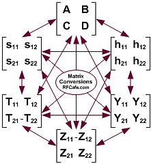
This article explains the six most common two-port network matrix descriptions
used in circuit theory, RF/microwave engineering, filter design, amplifier design,
and transmission-line analysis: Z-parameters, Y-parameters, h-parameters, ABCD-parameters,
S-parameters, and scattering-transfer T-parameters. Each representation describes
the same linear two-port network, but each chooses a different set of independent
and dependent variables. Because of that choice, some matrix types are natural for
low-frequency circuit analysis, some for cascade calculations, and some for high-frequency
measurement where direct open- and short-circuit tests become impractical.
The most important practical point is that there is no universally harmless conversion.
Many formulas contain denominators such as z21, y21, S21,
C, B, h21, h22, or matrix determinants. If one of these quantities
is zero or very small, the corresponding conversion may be singular or numerically
ill-conditioned, even though the physical network itself is perfectly valid. In
those cases, use another parameter set, take a limiting form, or use a robust numerical
matrix inversion method.
This report uses the standard two-port current convention in which I1
and I2 are currents entering their respective ports. For ABCD parameters,
the cascade-friendly convention is used:
V1 = A V2 - B I2
I1 = C V2
- D I2
or equivalently:
[ V1 ; I1 ] = [ [ A, B ], [ C, D ] ] [ V2 ;
-I2 ]
This sign convention is common in transmission-line and RF texts because it allows
cascaded two-port chains to be represented by ordinary matrix multiplication. However,
some books and software packages use a different ABCD sign convention. Always check
the convention before using a published formula.
For S-parameters and scattering-transfer T-parameters, this report assumes equal,
real reference impedances Z0 at both ports unless stated otherwise. Generalized
S-parameters with unequal or complex reference impedances require modified formulas
based on power-wave or pseudo-wave definitions. The power-wave formalism was introduced
by Kurokawa and remains important in precision RF metrology; see
Kurokawa, “Power Waves and the
Scattering Matrix,” IEEE Transactions on Microwave Theory and Techniques, 1965.
Key findings
- Z-parameters are impedance parameters. They express port voltages
as functions of port currents. They are intuitive for series impedances and low-frequency
circuit models, but their direct measurement requires open-circuit conditions.
- Y-parameters are admittance parameters. They express port currents
as functions of port voltages. They are convenient for nodal analysis, shunt elements,
and parallel connections, but their direct measurement requires short-circuit conditions.
- h-parameters are hybrid parameters. They mix voltage, current,
impedance, admittance, and dimensionless gain quantities. They were historically
popular for transistor small-signal models, especially at audio and radio frequencies.
- ABCD-parameters, also called transmission or chain parameters,
are especially useful for cascaded networks. The total ABCD matrix of a cascade
is the ordered product of the individual ABCD matrices.
- S-parameters are the standard high-frequency measurement parameters.
They relate incident and reflected traveling waves rather than port voltages and
currents. They are directly measured by vector network analyzers and are emphasized
in microwave engineering references such as Pozar’s
Microwave Engineering, Keysight’s
S-parameter application literature, and Rohde & Schwarz’s
S-parameter tutorials.
- Scattering-transfer T-parameters are wave-cascade parameters.
They are related to S-parameters but arranged so that cascaded RF/microwave networks
can be multiplied in chain order, much like ABCD matrices.
- Conversions are exact for linear two-port networks under the stated assumptions,
but the formulas can fail at singular cases. For example, conversion from S to T
requires S21 ≠ 0, and conversion from ABCD to Z using the common formulas
requires C ≠ 0.
- Reference impedance matters for S-parameters. A set of S-parameters is not complete
unless Z0 or the port reference impedances are specified.
Detailed analysis
1. Two-port network conventions used in this report
A two-port network has four terminal variables:
- V1: voltage at port 1
- I1: current entering port 1
- V2: voltage at port 2
- I2: current entering port 2
The current convention is important. In this report, both currents enter the
two-port. This is the usual network-theory convention for Z, Y, and h parameters.
For cascade work, however, the output current used in the ABCD equations is often
written as -I2, because the current leaving the first network enters
the next network. This gives the cascade-friendly form:
[ V1 ; I1 ] = [ [ A, B ], [ C, D ] ] [ V2 ;
-I2 ]
That is:
V1 = A V2 - B I2
I1 = C V2
- D I2
For S-parameters, define incident and reflected wave variables a1,
a2, b1, and b2. For equal real reference impedance
Z0:
an = (Vn + Z0In) / (2 sqrt(Z0))
bn = (Vn - Z0In) / (2 sqrt(Z0))
The S-parameter definition is:
[ b1 ; b2 ] = [ [ S11, S12 ], [ S21,
S22 ] ] [ a1 ; a2 ]
The scattering-transfer T-parameter definition used here is:
[ a1 ; b1 ] = [ [ T11, T12 ], [ T21,
T22 ] ] [ b2 ; a2 ]
This is one common RF chain-scattering convention, but not the only one. Some
references define a transfer matrix using [ b1 ; a1 ] or reverse
the port order. Therefore, when comparing formulas with software packages or textbooks,
verify the ordering of the wave variables. Tools such as
scikit-rf
and technical references such as
Qucs technical documentation
explicitly document their conventions.
2. Z-parameters: impedance parameters
Definition
Z-parameters express port voltages as linear functions of port currents:
[ V1 ; V2 ] = [ [ z11, z12 ], [ z21,
z22 ] ] [ I1 ; I2 ]
Expanded:
V1 = z11I1 + z12I2
V2 = z21I1 + z22I2
Parameter meanings
- z11 = V1 / I1 with I2 = 0. This
is the input impedance with port 2 open-circuited.
- z22 = V2 / I2 with I1 = 0. This
is the output impedance with port 1 open-circuited.
- z21 = V2 / I1 with I2 = 0. This
is the forward transfer impedance.
- z12 = V1 / I2 with I1 = 0. This
is the reverse transfer impedance.
Why use Z-parameters?
- They are intuitive when the network contains series impedances.
- They are convenient for low-frequency equivalent circuits.
- They connect directly with loop or mesh analysis.
- They are useful when open-circuit conditions are physically reasonable.
Limitations
Direct measurement of Z-parameters requires open-circuiting one port. At high
frequency, a physical open circuit is not ideal because it has stray capacitance
and radiates. Therefore, RF and microwave engineers usually measure S-parameters
instead and convert to Z-parameters if needed.
Example: series impedance
A simple series impedance Zs between port 1 and port 2 has an ABCD
matrix:
[ [ 1, Zs ], [ 0, 1 ] ]
It does not have a finite ordinary Z-parameter matrix in the same way as a general
two-port when the required open-circuit transfer conditions become singular. This
illustrates why not every parameter set is numerically well-behaved for every topology.
3. Y-parameters: admittance parameters
Definition
Y-parameters express port currents as linear functions of port voltages:
[ I1 ; I2 ] = [ [ y11, y12 ], [ y21,
y22 ] ] [ V1 ; V2 ]
Expanded:
I1 = y11V1 + y12V2
I2 = y21V1 + y22V2
Parameter meanings
- y11 = I1 / V1 with V2 = 0. This
is the input admittance with port 2 short-circuited.
- y22 = I2 / V2 with V1 = 0. This
is the output admittance with port 1 short-circuited.
- y21 = I2 / V1 with V2 = 0. This
is the forward transfer admittance.
- y12 = I1 / V2 with V1 = 0. This
is the reverse transfer admittance.
Why use Y-parameters?
- They are natural for nodal analysis.
- They are convenient for shunt elements and parallel network combinations.
- They are useful in small-signal transistor and active-device modeling.
- Admittance matrices combine directly for parallel-connected two-ports under
compatible port connections.
Limitations
Direct Y-parameter measurement requires short-circuit conditions. At RF and microwave
frequencies, a short circuit is also nonideal because it has inductance, finite
resistance, and fixture parasitics. Therefore, Y-parameters are often computed from
measured S-parameters.
4. h-parameters: hybrid parameters
Definition
h-parameters mix voltage and current variables:
[ V1 ; I2 ] = [ [ h11, h12 ], [ h21,
h22 ] ] [ I1 ; V2 ]
Expanded:
V1 = h11I1 + h12V2
I2 = h21I1 + h22V2
Parameter meanings
- h11 = V1 / I1 with V2 = 0. This
is an input impedance with output short-circuited.
- h12 = V1 / V2 with I1 = 0. This
is a reverse voltage ratio with input open-circuited.
- h21 = I2 / I1 with V2 = 0. This
is a forward current ratio with output short-circuited.
- h22 = I2 / V2 with I1 = 0. This
is an output admittance with input open-circuited.
Why use h-parameters?
- They historically fit transistor amplifier analysis well.
- h11 resembles input resistance, h21 resembles current
gain, h12 resembles reverse voltage feedback, and h22 resembles
output admittance.
- They are useful when one side of the network is naturally voltage-driven and
the other is naturally current-observed.
Limitations
h-parameters are less common in modern microwave work because open and short
test conditions are difficult at high frequency and because S-parameters are directly
measurable with a vector network analyzer. Also, h-parameter sign conventions can
be confusing because two-port network current directions may differ from transistor
data-sheet conventions.
5. ABCD-parameters: transmission or chain parameters
Definition
ABCD-parameters relate the input-port voltage and current to the output-port
voltage and the negative of output-port current:
[ V1 ; I1 ] = [ [ A, B ], [ C, D ] ] [ V2 ;
-I2 ]
Expanded:
V1 = A V2 - B I2
I1 = C V2
- D I2
Parameter meanings
- A = V1 / V2 with I2 = 0. This is a voltage
ratio with port 2 open-circuited.
- B = -V1 / I2 with V2 = 0. This has units of
ohms.
- C = I1 / V2 with I2 = 0. This has units of
siemens.
- D = -I1 / I2 with V2 = 0. This is a current
ratio.
Why use ABCD-parameters?
The main reason is cascading. Suppose network 1 feeds network 2. If each has
an ABCD matrix, the total cascade is:
[ABCD]total = [ABCD]1 [ABCD]2
For a chain of N networks:
[ABCD]total = [ABCD]1 [ABCD]2 ... [ABCD]N
The order matters. Matrix multiplication is generally not commutative.
Common ABCD building blocks
| Network element |
ABCD matrix |
Comment |
| Series impedance Z |
[ [ 1, Z ], [ 0, 1 ] ] |
Useful for series resistors, inductors, capacitors, and transmission-line approximations. |
| Shunt admittance Y |
[ [ 1, 0 ], [ Y, 1 ] ] |
Useful for shunt capacitors, inductors, conductances, and stubs. |
| Lossless transmission line, length l |
[ [ cos(βl), jZ0sin(βl) ], [ j(1/Z0)sin(βl),
cos(βl) ] ] |
For a lossless line with characteristic impedance Z0. |
| General transmission line |
[ [ cosh(γl), Zcsinh(γl) ], [ (1/Zc)sinh(γl),
cosh(γl) ] ] |
For propagation constant γ and characteristic impedance Zc. |
Transmission-line ABCD formulas are standard in microwave network theory; see
Pozar’s
Microwave Engineering and the open microwave network text by Steer at
LibreTexts.
Step-by-step cascade example
Suppose a network consists of a series impedance Z1, then a shunt
admittance Y2, then a series impedance Z3. The individual
ABCD matrices are:
M1 = [ [ 1, Z1 ], [ 0, 1 ] ]
M2 = [ [ 1,
0 ], [ Y2, 1 ] ]
M3 = [ [ 1, Z3 ], [ 0, 1 ]
]
The total matrix is:
Mtotal = M1M2M3
First multiply M1M2:
M12 = [ [ 1 + Z1Y2, Z1 ], [ Y2,
1 ] ]
Then multiply by M3:
Mtotal = [ [ 1 + Z1Y2, Z1 + Z3
+ Z1Y2Z3 ], [ Y2, 1 + Y2Z3
] ]
Thus:
A = 1 + Z1Y2
B = Z1 + Z3 + Z1Y2Z3
C = Y2
D = 1 + Y2Z3
6. S-parameters: scattering parameters
Definition
S-parameters relate reflected waves to incident waves:
[ b1 ; b2 ] = [ [ S11, S12 ], [ S21,
S22 ] ] [ a1 ; a2 ]
Expanded:
b1 = S11a1 + S12a2
b2 = S21a1 + S22a2
Parameter meanings
- S11: input reflection coefficient with port 2 terminated in Z0.
- S22: output reflection coefficient with port 1 terminated in Z0.
- S21: forward transmission coefficient or gain from port 1 to port
2.
- S12: reverse transmission coefficient or isolation from port 2 to
port 1.
Why use S-parameters?
- They are directly measurable at RF and microwave frequencies with a vector network
analyzer.
- They avoid requiring ideal open and short circuits at the device ports.
- They naturally describe reflection, insertion loss, gain, return loss, and isolation.
- They are widely used in data files such as Touchstone files.
Industry measurement practice is strongly centered on S-parameters; see Keysight’s
S-parameter application note and Rohde & Schwarz’s
S-parameter overview.
Important S-parameter quantities
- Return loss at port 1: RL1 = -20 log10|S11|
dB
- Insertion loss for a passive forward path: IL = -20 log10|S21|
dB
- Forward gain: G = 20 log10|S21| dB, when the network is
active or has gain
- Reverse isolation: ISO = -20 log10|S12| dB
Limitations
S-parameters depend on the reference impedance. A two-port’s S-parameters at
50 ohms are not generally the same as its S-parameters at 75 ohms. Also, for strongly
nonlinear devices, ordinary small-signal S-parameters are valid only around a specified
bias point and signal level.
7. Scattering-transfer T-parameters: wave chain parameters
Definition used here
[ a1 ; b1 ] = [ [ T11, T12 ], [ T21,
T22 ] ] [ b2 ; a2 ]
Why use scattering-transfer T-parameters?
- They allow cascaded RF networks to be multiplied directly.
- They are useful when measured networks are available as S-parameters but must
be cascaded many times.
- They avoid repeated S-to-ABCD-to-S conversions in some microwave calculations.
If network 1 feeds network 2, and both are represented by compatible scattering-transfer
matrices, then:
Ttotal = T1T2
Caution
Conversion from S to this T form requires S21 ≠ 0. If S21
is zero or extremely small, the T matrix becomes singular or numerically very large.
This often happens near transmission zeros, which are common in filters. In such
cases, a direct S-matrix cascade method or a different parameter set may be more
numerically stable.
8. Reciprocity, symmetry, and losslessness
Reciprocity
For a reciprocal two-port under the conventions used here:
- Z-parameters: z12 = z21
- Y-parameters: y12 = y21
- ABCD-parameters: AD - BC = 1
- S-parameters with equal reference impedances: S12 = S21
Symmetry
A physically symmetric two-port has the same behavior looking into either port.
Common tests include:
- Z-parameters: z11 = z22
- Y-parameters: y11 = y22
- ABCD-parameters: A = D
- S-parameters with equal reference impedances: S11 = S22
Losslessness
For a passive lossless two-port with real equal reference impedances, the S-matrix
is unitary:
S†S = I
where S† is the conjugate transpose of S. This implies conservation
of incident and reflected power. The unitarity property is one reason S-parameters
are so useful in microwave engineering.
9. Notation for conversion formulas
The following determinants and abbreviations are used throughout the conversion
tables:
ΔZ = z11z22 - z12z21
ΔY = y11y22 - y12y21
Δh = h11h22 - h12h21
ΔA = AD - BC
ΔS = S11S22 - S12S21
ΔT = T11T22 - T12T21
Z0 is the real reference impedance for S and T parameters. Y0
= 1 / Z0.
All formulas assume that the displayed denominators are nonzero. If a denominator
is zero, the conversion may not exist in that form.
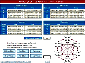
10. Core conversion table
The table below gives explicit conversions among Z, Y, h, ABCD, S, and scattering-transfer
T parameters under the conventions stated above. For compactness, some cells use
an intermediate conversion. That is still an explicit formula: compute the intermediate
quantities shown, then substitute them into the stated target formula.
| From / To |
Z |
Y |
h |
ABCD |
S |
T |
| Z |
Identity |
y11 = z22/ΔZ
y12 = -z12/ΔZ
y21 = -z21/ΔZ
y22 = z11/ΔZ
|
h11 = ΔZ/z22
h12 = z12/z22
h21 = -z21/z22
h22 = 1/z22
|
A = z11/z21
B = ΔZ/z21
C = 1/z21
D = z22/z21 |
Let DZS = (z11 + Z0)(z22 + Z0)
- z12z21.
S11 = ((z11 - Z0)(z22
+ Z0) - z12z21)/DZS
S12
= 2Z0z12/DZS
S21 = 2Z0z21/DZS
S22 = ((z22 - Z0)(z11 + Z0)
- z12z21)/DZS |
First compute ABCD:
A = z11/z21, B = ΔZ/z21,
C = 1/z21, D = z22/z21.
Then:
T11
= (A + B/Z0 + CZ0 + D)/2
T12 = (A - B/Z0
+ CZ0 - D)/2
T21 = (A + B/Z0 - CZ0
- D)/2
T22 = (A - B/Z0 - CZ0 + D)/2 |
| Y |
z11 = y22/ΔY
z12 = -y12/ΔY
z21 = -y21/ΔY
z22 = y11/ΔY
|
Identity |
h11 = 1/y11
h12 = -y12/y11
h21 = y21/y11
h22 = ΔY/y11
|
A = -y22/y21
B = -1/y21
C = -ΔY/y21
D = -y11/y21 |
Let DYS = (y11 + Y0)(y22 + Y0)
- y12y21.
S11 = ((Y0 - y11)(Y0
+ y22) + y12y21)/DYS
S12
= -2Y0y12/DYS
S21 = -2Y0y21/DYS
S22 = ((Y0 + y11)(Y0 - y22)
+ y12y21)/DYS |
First compute ABCD:
A = -y22/y21, B = -1/y21,
C = -ΔY/y21, D = -y11/y21.
Then use:
T11 = (A + B/Z0 + CZ0 + D)/2
T12
= (A - B/Z0 + CZ0 - D)/2
T21 = (A + B/Z0
- CZ0 - D)/2
T22 = (A - B/Z0 - CZ0
+ D)/2 |
| h |
z11 = Δh/h22
z12 = h12/h22
z21 = -h21/h22
z22 = 1/h22
|
y11 = 1/h11
y12 = -h12/h11
y21 = h21/h11
y22 = Δh/h11
|
Identity |
A = -Δh/h21
B = -h11/h21
C = -h22/h21
D = -1/h21 |
Let NhS = (Δh + Z0h22)(1 +
Z0h22) + h12h21.
S11 =
((Δh - Z0h22)(1 + Z0h22)
+ h12h21)/NhS
S12 = 2Z0h12h22/NhS
S21 = -2Z0h21h22/NhS
S22
= ((1 - Z0h22)(Δh + Z0h22)
+ h12h21)/NhS |
First compute ABCD:
A = -Δh/h21, B = -h11/h21,
C = -h22/h21, D = -1/h21.
Then:
T11
= (A + B/Z0 + CZ0 + D)/2
T12 = (A - B/Z0
+ CZ0 - D)/2
T21 = (A + B/Z0 - CZ0
- D)/2
T22 = (A - B/Z0 - CZ0 + D)/2 |
| ABCD |
z11 = A/C
z12 = ΔA/C
z21
= 1/C
z22 = D/C |
y11 = D/B
y12 = -ΔA/B
y21
= -1/B
y22 = A/B |
h11 = B/D
h12 = ΔA/D
h21
= -1/D
h22 = C/D |
Identity |
Let DAS = A + B/Z0 + CZ0 + D.
S11
= (A + B/Z0 - CZ0 - D)/DAS
S21 =
2/DAS
S12 = 2ΔA/DAS
S22
= (-A + B/Z0 - CZ0 + D)/DAS |
T11 = (A + B/Z0 + CZ0 + D)/2
T12
= (A - B/Z0 + CZ0 - D)/2
T21 = (A + B/Z0
- CZ0 - D)/2
T22 = (A - B/Z0 - CZ0
+ D)/2 |
| S |
Let DSZ = (1 - S11)(1 - S22) - S12S21.
z11 = Z0((1 + S11)(1 - S22) + S12S21)/DSZ
z12 = 2Z0S12/DSZ
z21 =
2Z0S21/DSZ
z22 = Z0((1
- S11)(1 + S22) + S12S21)/DSZ
|
Let DSY = (1 + S11)(1 + S22) - S12S21.
y11 = Y0((1 - S11)(1 + S22) + S12S21)/DSY
y12 = -2Y0S12/DSY
y21
= -2Y0S21/DSY
y22 = Y0((1
+ S11)(1 - S22) + S12S21)/DSY
|
Let NSh = (1 - S11)(1 + S22) + S12S21.
Let DSZ = (1 - S11)(1 - S22) - S12S21.
h11 = Z0((1 + S11)(1 + S22) - S12S21)/NSh
h12 = 2S12/NSh
h21 = -2S21/NSh
h22 = DSZ/(Z0NSh) |
A = ((1 + S11)(1 - S22) + S12S21)/(2S21)
B = Z0((1 + S11)(1 + S22) - S12S21)/(2S21)
C = ((1 - S11)(1 - S22) - S12S21)/(2Z0S21)
D = ((1 - S11)(1 + S22) + S12S21)/(2S21)
|
Identity |
T11 = 1/S21
T12 = -S22/S21
T21 = S11/S21
T22 = -ΔS/S21
|
| T |
First compute S:
S11 = T21/T11
S21
= 1/T11
S12 = ΔT/T11
S22
= -T12/T11
Then use the S-to-Z formulas. |
First compute S:
S11 = T21/T11
S21
= 1/T11
S12 = ΔT/T11
S22
= -T12/T11
Then use the S-to-Y formulas. |
First compute S:
S11 = T21/T11
S21
= 1/T11
S12 = ΔT/T11
S22
= -T12/T11
Then use the S-to-h formulas. |
A = (T11 + T12 + T21 + T22)/2
B = Z0(T11 - T12 + T21 - T22)/2
C = (T11 + T12 - T21 - T22)/(2Z0)
D = (T11 - T12 - T21 + T22)/2 |
S11 = T21/T11
S21 = 1/T11
S12 = ΔT/T11
S22 = -T12/T11
|
Identity |
11. Step-by-step method for using the conversion formulas
- Identify the source parameter set. For example, determine whether
your data are Z, Y, h, ABCD, S, or T parameters.
- Verify the convention. This is especially important for ABCD
and T parameters. Confirm the current direction and the ordering of variables.
- Write down the known matrix elements. For example, if you have
S-parameters, list S11, S12, S21, and S22.
- Check the reference impedance. For S and T conversions, identify
Z0. Common values are 50 ohms and 75 ohms.
- Compute any determinant or denominator. For example, when converting
S to Z, compute DSZ = (1 - S11)(1 - S22) - S12S21.
- Check for singular or nearly singular denominators. If a denominator
is zero or very small, the formula may produce a misleading result.
- Apply the formula element by element. Keep complex arithmetic
intact; phase matters.
- Check units. Z elements are in ohms, Y elements are in siemens,
B is in ohms, C is in siemens, while A, D, S, and T elements are generally dimensionless.
- Validate the result with known physical properties. For a reciprocal
passive two-port, check z12 = z21, y12 = y21,
S12 = S21, or AD - BC = 1, as applicable.
12. Practical application guidance
Use Z-parameters when:
- The circuit is low-frequency and naturally described by impedances.
- Series elements dominate.
- You are doing mesh analysis.
- Open-circuit test conditions are reasonable.
Use Y-parameters when:
- The circuit is naturally described by shunt admittances.
- Nodal analysis is convenient.
- Parallel connection of networks is being studied.
- Short-circuit test conditions are reasonable.
Use h-parameters when:
- You are analyzing transistor small-signal amplifier stages in classical low-frequency
form.
- You want current gain and input impedance to appear directly in the model.
- You are working from older transistor data sheets or educational material.
Use ABCD-parameters when:
- The network is a cascade of two-port blocks.
- You are analyzing filters, attenuator pads, matching networks, or transmission-line
sections.
- You want the total response of a chain by matrix multiplication.
Use S-parameters when:
- You are working at RF, microwave, or millimeter-wave frequencies.
- The network is measured with a vector network analyzer.
- You care about return loss, insertion loss, gain, isolation, or match.
- You are exchanging device data using Touchstone files.
Use scattering-transfer T-parameters when:
- You have S-parameter data but need to cascade multiple networks.
- You want wave-based cascade calculations.
- You are careful about transmission zeros where S21 may approach zero.
13. Worked example: converting ABCD to S
Suppose a two-port has ABCD parameters A, B, C, and D and is used in a 50-ohm
system. Let Z0 = 50 ohms.
Step 1: Compute the common denominator:
DAS = A + B/50 + 50C + D
Step 2: Compute input reflection:
S11 = (A + B/50 - 50C - D)/DAS
Step 3: Compute forward transmission:
S21 = 2/DAS
Step 4: Compute reverse transmission:
S12 = 2(AD - BC)/DAS
Step 5: Compute output reflection:
S22 = (-A + B/50 - 50C + D)/DAS
If the network is reciprocal, AD - BC = 1, so S12 = S21
for equal reference impedances.
14. Worked example: converting S to ABCD
Suppose measured S-parameters are available from a vector network analyzer and
you want to cascade the device with other circuit blocks. Use the S-to-ABCD formulas.
Step 1: Confirm Z0. If the measurement was made in a 50-ohm system,
Z0 = 50 ohms.
Step 2: Confirm S21 is not zero. The standard S-to-ABCD formula divides
by S21.
Step 3: Compute:
A = ((1 + S11)(1 - S22) + S12S21)/(2S21)
B = Z0((1 + S11)(1 + S22) - S12S21)/(2S21)
C = ((1 - S11)(1 - S22) - S12S21)/(2Z0S21)
D = ((1 - S11)(1 + S22) + S12S21)/(2S21)
Step 4: Cascade by multiplying ABCD matrices in the physical order of the signal
path.
15. Numerical and physical cautions
Singular conversions
A conversion may be singular even when the physical network is well-defined.
Examples:
- Z to ABCD formula above requires z21 ≠ 0.
- Y to ABCD formula above requires y21 ≠ 0.
- ABCD to Z formula above requires C ≠ 0.
- ABCD to Y formula above requires B ≠ 0.
- S to ABCD and S to T require S21 ≠ 0.
- T to S requires T11 ≠ 0.
Near-zero denominators
If a denominator is very small, the conversion may amplify measurement noise.
This is especially important when converting measured S-parameters near filter transmission
zeros. In those cases, the converted ABCD or T values may become very large even
though the original S-parameters are physically meaningful.
Reference impedance and renormalization
S-parameters must specify their reference impedance. If a device measured at
50 ohms is placed in a 75-ohm system, the S-parameters should be renormalized or
converted through Z/Y parameters and then re-expressed at the new reference impedance.
Modern RF tools implement this, but the underlying mathematics depends on the wave
definition and reference impedance convention.
Complex reference impedances
The formulas in this report assume equal real Z0. For unequal or complex
reference impedances, use generalized formulas. This is not merely a cosmetic change:
the definition of wave amplitude affects power normalization, conjugation, and passivity
tests. Kurokawa’s power-wave
paper is the classic reference.
Open questions / debates in the field
- ABCD and T convention differences: There is no single universal
notation for chain matrices. Some authors define ABCD using I2 instead
of -I2. Some define scattering transfer matrices with different wave
ordering. This is not a scientific dispute, but it is a persistent source of engineering
errors.
- Power waves versus pseudo-waves: For complex reference impedances,
different wave definitions can give different-looking S-parameters. The correct
choice depends on whether the goal is power accounting, measurement calibration,
or mathematical convenience.
- Numerical stability in cascades: Cascading many networks using
ABCD or T matrices can lead to very large or very small numbers, especially for
long lossy lines or high-rejection filters. Engineers debate and develop more stable
algorithms, including Redheffer star products and state-space approaches.
- Passivity and causality enforcement: Measured broadband S-parameters
often contain small errors that violate passivity or causality. Correcting those
data without distorting the real device behavior is an active topic in RF/microwave
modeling and signal-integrity work.
- Linear versus nonlinear behavior: Ordinary two-port matrices
describe linear small-signal behavior. Power amplifiers, mixers, varactors, and
switching devices may require X-parameters, large-signal S-parameters, harmonic-balance
models, or time-domain nonlinear models.
- De-embedding and fixture removal: Converting among matrices
is straightforward in theory, but real measurements include fixtures, launches,
connectors, and calibration standards. The best de-embedding method depends on the
frequency range, substrate, calibration quality, and device geometry.
Sources cited and useful references
- David M. Pozar,
Microwave Engineering, Wiley. Standard academic microwave engineering text covering
S-parameters, transmission lines, and two-port networks.
- Keysight Technologies,
S-Parameter Design Application Note. Industry reference for S-parameter concepts
and measurement usage.
- Rohde & Schwarz,
Understanding S-Parameters. Industry tutorial on scattering parameters and RF
measurement interpretation.
- Qucs Project, Technical Documentation
on Network Parameter Conversions. Open technical documentation containing two-port
conversion formulas and circuit-simulation conventions.
- scikit-rf Project,
Network
Tutorial Documentation. Practical open-source RF/microwave network-analysis
documentation.
- David M. Pozar and other microwave engineering texts commonly derive ABCD-to-S
and S-to-ABCD formulas using equal real reference impedance; the same relationships
are also summarized in many RF CAD tool manuals.
- Kaneyuki Kurokawa, “Power
Waves and the Scattering Matrix,” IEEE Transactions on Microwave Theory and Techniques,
1965. Classic paper on power-wave definitions for scattering matrices.
- Michael Steer,
Microwave and RF Design: Networks, Two-Port Networks, LibreTexts. Open educational
reference on two-port network descriptions.
Final practical advice
For hand analysis, choose the parameter set that matches the circuit structure:
Z for series behavior, Y for shunt behavior, ABCD for cascades, and h for classical
transistor models. For RF measurement, begin with S-parameters because they are
what the instrument directly measures. Convert only when the target representation
gives a clear advantage, and always check the sign convention, reference impedance,
and singular denominators before trusting the result.
 This content was generated primarily with
the assistance of ChatGPT (OpenAI), and/or
Gemini (Google), and/or
Arya (GabAI), and/or Grok
(x.AI), and/or DeepSeek artificial intelligence
(AI) engines. Review was performed to help detect and correct any inaccuracies;
however, you are encouraged to verify the information yourself if it will be used
for critical applications. In all cases, multiple solicitations to the AI engine(s)
was(were) used to assimilate final content. Images and external hyperlinks have
also been added occasionally - especially on extensive treatises. Courts have ruled
that AI-generated content is not subject to copyright restrictions, but since I
modify them, everything here is protected by RF Cafe copyright. Many of the images
are likewise generated and modified. Your use of this data implies an agreement
to hold totally harmless Kirt Blattenberger, RF Cafe, and any and all of its assigns.
Thank you. Here is Gab AI in an iFrame. This content was generated primarily with
the assistance of ChatGPT (OpenAI), and/or
Gemini (Google), and/or
Arya (GabAI), and/or Grok
(x.AI), and/or DeepSeek artificial intelligence
(AI) engines. Review was performed to help detect and correct any inaccuracies;
however, you are encouraged to verify the information yourself if it will be used
for critical applications. In all cases, multiple solicitations to the AI engine(s)
was(were) used to assimilate final content. Images and external hyperlinks have
also been added occasionally - especially on extensive treatises. Courts have ruled
that AI-generated content is not subject to copyright restrictions, but since I
modify them, everything here is protected by RF Cafe copyright. Many of the images
are likewise generated and modified. Your use of this data implies an agreement
to hold totally harmless Kirt Blattenberger, RF Cafe, and any and all of its assigns.
Thank you. Here is Gab AI in an iFrame.
Electronics & High Tech
Companies | Electronics &
Tech Publications | Electronics &
Tech Pioneers | Electronics &
Tech Principles |
Tech Standards Groups &
Industry Associations | Societal
Influences on Technology
|