Voltage Standing Wave Ratio (VSWR) - Its History, Meaning, and Calculation^©

By Kirt Blattenberger, RF Engineer, RFCafe.com webmaster

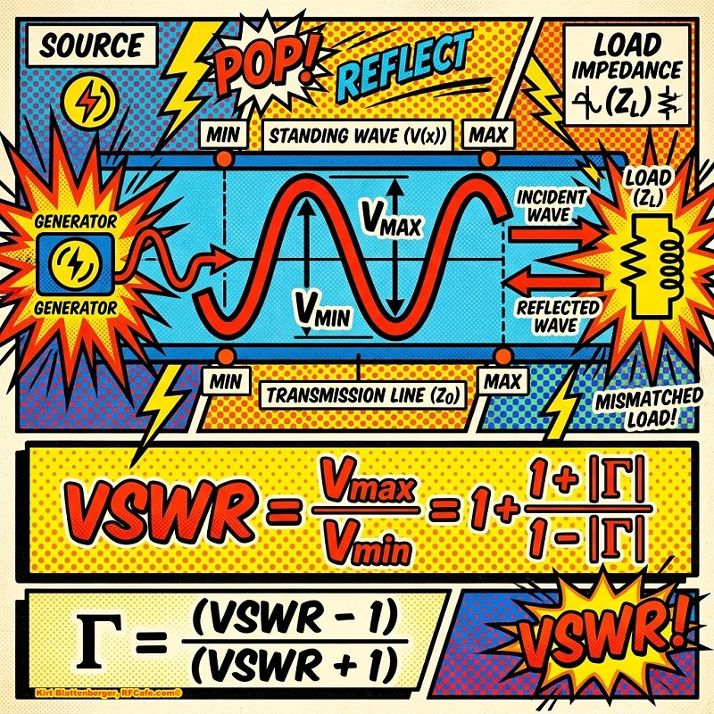
1. Executive Summary

Voltage standing wave ratio (VSWR), often shortened to SWR in radio work, is a measure of how well a load impedance is matched to a transmission line. It is defined as the ratio of the maximum RF voltage to the minimum RF voltage along a transmission line when forward and reflected waves interfere:

VSWR = V_max / V_min = (1 + |Γ|) / (1 - |Γ|)

where Γ, the reflection coefficient, is the complex ratio of reflected voltage wave to incident voltage wave. A perfect match has Γ = 0 and VSWR = 1:1. An open circuit or short circuit has |Γ| = 1 and VSWR is infinite. In practical RF systems, VSWR is a convenient scalar indication of mismatch, but it does not by itself show the phase of the reflection, the actual impedance, or the location of the mismatch. For those purposes, engineers use the complex reflection coefficient, impedance calculations, time-domain methods, or graphical tools such as the Smith Chart.

The modern theory behind VSWR comes from the development of transmission-line theory during the 19th and early 20th centuries. James Clerk Maxwell in Cambridge, England, provided the electromagnetic foundation; Oliver Heaviside in England developed the telegrapher's equations and practical transmission-line analysis; Heinrich Hertz in Karlsruhe, Germany, experimentally demonstrated electromagnetic waves and standing waves; and Phillip H. Smith at Bell Telephone Laboratories in New Jersey, USA, created the Smith Chart in the 1930s as a practical graphical tool for impedance and reflection-coefficient analysis. The concept itself was not invented by one person in one place; it emerged from wave theory, telegraph-line engineering, and radio-frequency measurement practice.

VSWR is central in RF engineering because impedance mismatch causes reflected power, standing waves, increased voltage and current stress, transmitter foldback or damage, measurement uncertainty, and frequency-dependent amplitude and phase ripple. In broadband systems, mismatch ripple can distort the amplitude and phase of signals across the passband and can produce group-delay ripple, which is especially important in radar, communication, instrumentation, and high-speed digital systems.

For precision measurement, a vector network analyzer (VNA) must be calibrated so that measured reflection and transmission data represent the device under test rather than the analyzer, cables, adapters, and test fixtures. Short-Open-Load-Through calibration, commonly called SOLT calibration, uses known short, open, load, and through standards to characterize and mathematically remove systematic VNA errors such as directivity, source match, load match, reflection tracking, and transmission tracking. SOLT is one of the most common coaxial VNA calibration methods and is especially useful when accurate, connectorized standards are available.

2. Key Findings

• VSWR is a scalar measure of standing-wave severity on a transmission line. It is determined only by the magnitude of the reflection coefficient, |Γ|, not by its phase.

• The reflection coefficient at a load is:

Γ_L = (Z_L - Z₀) / (Z_L + Z₀)

where Z_L is load impedance and Z₀ is characteristic impedance.

• A perfect line termination occurs when Z_L = Z₀. Then Γ = 0, reflected power is zero, and VSWR = 1:1.

• For maximum real power transfer from a source with complex internal impedance Z_S = R_S + jX_S, the load must be the complex conjugate:

Z_L = Z_S^* = R_S - jX_S

This is often called conjugate matching. It cancels net reactance and makes the load resistance equal to the source resistance.

• The terms "reciprocal impedance" and "conjugate impedance" are sometimes confused. Strictly, reciprocal usually means 1/Z or bilateral network behavior, while maximum power transfer requires the complex conjugate, not the mathematical reciprocal.

• VSWR is related to return loss, reflected power, and mismatch loss. For example, a VSWR of 2:1 corresponds to |Γ| = 0.333, return loss of about 9.54 dB, and reflected power of about 11.1%.

• The Smith Chart maps complex impedance and reflection coefficient onto one graphical plane. It turns difficult complex arithmetic into geometric operations: impedance transformation along a line becomes rotation around the chart, and constant VSWR corresponds to a circle centered on the chart origin.

• Mismatch between source, line, and load causes multiple reflections. These reflections create frequency-dependent amplitude ripple and phase ripple. In broadband signals, this can become waveform distortion and group-delay variation.

• SOLT VNA calibration is necessary when accurate measurement of VSWR, S-parameters, impedance, return loss, and insertion loss is required. It compensates for systematic errors caused by imperfect analyzers, cables, adapters, connectors, and fixtures.

• Historical attribution is shared: Maxwell, Heaviside, Hertz, Rayleigh, Kennelly, Pupin, Campbell, Carson, Smith, and others contributed to the wave, transmission-line, and impedance-analysis framework that makes modern VSWR analysis possible.

3. Detailed Analysis

3.1 What VSWR Means Physically

A transmission line carries electromagnetic energy from a source to a load. If the load impedance equals the characteristic impedance of the line, all forward-traveling power is absorbed by the load, except for line loss. No reflected wave is produced.

If the load impedance does not equal the line impedance, the load cannot absorb the incident wave in the exact voltage-current ratio imposed by the line. A reflected wave is generated. The forward and reflected waves add vectorially along the line. At some points they reinforce, producing voltage maxima; at other points they partially cancel, producing voltage minima. The ratio of these two values is the voltage standing wave ratio:

VSWR = V_max / V_min

VSWR is normally written as "N:1." Thus, VSWR = 1 means 1:1, VSWR = 2 means 2:1, and so on.

A VSWR of 1:1 is ideal. A higher value means greater mismatch. However, whether a given VSWR is acceptable depends on application. A 2:1 VSWR may be acceptable in many amateur-radio antenna systems, while precision microwave measurement systems may require much better matching. High-power transmitters, radar systems, satellite links, and low-noise microwave receivers may have much stricter requirements.

3.2 Historical Development: People and Places

James Clerk Maxwell — Cambridge, England
James Clerk Maxwell established the electromagnetic field theory that made transmission-line and wave analysis possible. His equations predicted electromagnetic waves traveling at approximately the speed of light. Maxwell's work appeared in the 1860s and was later collected in A Treatise on Electricity and Magnetism. A public copy is available through the Internet Archive: Maxwell, A Treatise on Electricity and Magnetism.

Oliver Heaviside — England
Oliver Heaviside reformulated Maxwell's equations into a more practical vector form and developed the telegrapher's equations for voltage and current on transmission lines. His work was essential for understanding long telegraph and telephone lines as distributed-parameter systems rather than simple lumped circuits. Heaviside's Electromagnetic Theory is available through the Internet Archive: Heaviside, Electromagnetic Theory.

Heinrich Hertz — Karlsruhe, Germany
Heinrich Hertz experimentally demonstrated electromagnetic waves in the late 1880s. His experiments in Karlsruhe showed reflection, refraction, interference, polarization, and standing-wave behavior. Hertz's work confirmed Maxwell's predictions and directly connected electromagnetic waves with laboratory-observable standing waves. See the Nobel Prize background discussion of Hertz's influence: Nobel Prize: Wireless Telegraphy and Hertzian Waves.

Lord Rayleigh — United Kingdom
Lord Rayleigh, born John William Strutt, contributed broadly to wave theory, acoustics, optics, and electrical transmission. His analyses of waves, reflection, resonance, and energy flow helped shape the mathematical environment in which transmission-line theory developed. Many reflection and wave concepts used in RF engineering have analogs in acoustics and optics.

Arthur E. Kennelly — United States
Arthur Edwin Kennelly contributed to alternating-current theory, complex impedance usage, and transmission-line engineering. He was associated with Harvard University and MIT and helped popularize complex-number methods in AC circuit analysis. Complex impedance is fundamental to reflection-coefficient and VSWR analysis.

Michael I. Pupin and George A. Campbell — Columbia University and Bell System, United States
Pupin and Campbell independently contributed to loaded telephone-line theory around the turn of the 20th century. Their work on practical long-distance lines helped establish the importance of characteristic impedance, propagation constant, attenuation, and line loading. Campbell worked for AT&T/Bell System. Pupin was at Columbia University in New York. Their work is part of the engineering lineage leading to modern transmission-line practice.

John R. Carson — Bell Telephone Laboratories, New York/New Jersey, United States
John Renshaw Carson made major contributions to communication theory, modulation, and transmission-line analysis. Bell System research provided much of the early industrial foundation for RF, microwave, coaxial-line, and network-analysis techniques.

Phillip H. Smith — Bell Telephone Laboratories, New Jersey, United States
Phillip Hagar Smith developed the Smith Chart while working at Bell Telephone Laboratories. The chart appeared in the late 1930s as a practical way to solve transmission-line and impedance-matching problems graphically. Smith's classic paper is "Transmission Line Calculator," Electronics, 1939. A later paper, "An Improved Transmission Line Calculator," appeared in Proceedings of the IRE. A historical overview is provided by the IEEE History Center: IEEE Engineering and Technology History Wiki: Smith Chart.

Kaneyuki Kurokawa — Bell Telephone Laboratories, United States
Kurokawa's later work on power waves and scattering parameters clarified how power, impedance, and reflection should be treated when reference impedances are complex. His 1965 paper "Power Waves and the Scattering Matrix" is important in advanced microwave network theory. See IEEE Xplore entry: Kurokawa, Power Waves and the Scattering Matrix.

Important Historical Caution
No single inventor can be credited with "inventing VSWR." Standing waves were known in wave physics before radio-frequency engineering matured. VSWR as a measurement quantity emerged from transmission-line practice, slotted-line measurements, impedance-matching work, and microwave engineering. The modern analysis process is a synthesis of electromagnetic theory, telegrapher's equations, complex impedance, reflection coefficient, and network theory.

3.3 Transmission-Line Model

A uniform transmission line is described by distributed resistance R, inductance L, conductance G, and capacitance C per unit length. The telegrapher's equations for sinusoidal steady state are:

dV/dz = -(R + jωL) I
dI/dz = -(G + jωC) V

where:

V = phasor voltage
I = phasor current
z = distance along the line
R = series resistance per unit length
L = series inductance per unit length
G = shunt conductance per unit length
C = shunt capacitance per unit length
ω = angular frequency = 2πf
j = square root of -1

Solving these equations gives traveling waves:

V(z) = V⁺ e^-γz + V^- e^+γz

I(z) = (V⁺/Z₀) e^-γz - (V^-/Z₀) e^+γz

where:

V⁺ = forward-traveling voltage-wave amplitude
V^- = reflected voltage-wave amplitude
γ = propagation constant = α + jβ
α = attenuation constant, in nepers per unit length
β = phase constant, in radians per unit length
Z₀ = characteristic impedance of the line

The characteristic impedance is:

Z₀ = sqrt((R + jωL) / (G + jωC))

For an ideal lossless line, R = 0 and G = 0, so:

Z₀ = sqrt(L/C)

In common RF coaxial systems, Z₀ is often 50 ohms. In television and cable systems, 75 ohms is common. Other values exist in balanced lines, waveguides, IC interconnects, and special-purpose systems.

3.4 Derivation of Reflection Coefficient

At the load, define the load impedance:

Z_L = V_L / I_L

At the load plane, the total voltage is the sum of forward and reflected voltages:

V_L = V⁺ + V^-

The total current is the forward current minus the reflected current, because the reflected wave travels in the opposite direction:

I_L = V⁺/Z₀ - V^-/Z₀

Therefore:

Z_L = (V⁺ + V^-) / ((V⁺/Z₀) - (V^-/Z₀))

Define the load reflection coefficient:

Γ_L = V^- / V⁺

Substitute:

Z_L = Z₀ (1 + Γ_L) / (1 - Γ_L)

Solving for Γ_L:

Γ_L = (Z_L - Z₀) / (Z_L + Z₀)

This is one of the most important equations in RF engineering.

3.5 Derivation of VSWR from Reflection Coefficient

On a lossless line, the forward and reflected voltages add as phasors. At a voltage maximum, they are in phase:

V_max = |V⁺| + |V^-|

At a voltage minimum, they are opposite in phase:

V_min = |V⁺| - |V^-|

Since |Γ| = |V^-| / |V⁺|:

VSWR = V_max / V_min

VSWR = (|V⁺| + |V^-|) / (|V⁺| - |V^-|)

Divide numerator and denominator by |V⁺|:

VSWR = (1 + |Γ|) / (1 - |Γ|)

Solving for |Γ|:

|Γ| = (VSWR - 1) / (VSWR + 1)

3.6 Reflected Power, Return Loss, and Mismatch Loss

The fraction of incident power reflected by a load is:

P_reflected / P_incident = |Γ|²

The fraction of incident power delivered to the load, assuming a lossless line and passive load, is:

P_delivered / P_incident = 1 - |Γ|²

Return loss is a positive dB quantity expressing how small the reflection is:

Return Loss = -20 log₁₀|Γ| dB

Equivalently:

Return Loss = 20 log₁₀(1/|Γ|) dB

Mismatch loss is the loss of available incident power due to reflection:

Mismatch Loss = -10 log₁₀(1 - |Γ|²) dB

These definitions are widely used in RF and microwave practice; see Keysight's network-analysis application material: Keysight, Understanding the Fundamental Principles of Vector Network Analysis.

3.7 Important Distinction: VSWR Does Not Fully Define Impedance

VSWR depends only on |Γ|. It does not reveal the angle of Γ. Many different load impedances can have the same VSWR.

Example in a 50-ohm system:

If VSWR = 2:1, then:

|Γ| = (2 - 1) / (2 + 1) = 1/3 = 0.333

One possible load is purely resistive and high:

Z_L = 100 ohms

Then:

Γ = (100 - 50) / (100 + 50) = 50/150 = +0.333

Another possible load is purely resistive and low:

Z_L = 25 ohms

Then:

Γ = (25 - 50) / (25 + 50) = -25/75 = -0.333

Both have |Γ| = 0.333 and VSWR = 2:1, but their reflection phases differ by 180 degrees. A VSWR meter alone cannot distinguish these cases.

3.8 Complex Impedance and Conjugate Matching

In AC and RF systems, impedance is generally complex:

Z = R + jX

where:

R = resistance, the real part, which dissipates or receives real power
X = reactance, the imaginary part, which stores and returns energy
jX = inductive if X is positive, capacitive if X is negative

A source may be modeled as an ideal voltage source V_S in series with source impedance:

Z_S = R_S + jX_S

The load is:

Z_L = R_L + jX_L

The average real power delivered to the load is maximized when:

Z_L = Z_S^* = R_S - jX_S

This is the complex-conjugate match condition.

Derivation of Maximum Power Transfer for Complex Impedances

Let the source voltage be V_S RMS. The current is:

I = V_S / (Z_S + Z_L)

The average power delivered to the load resistance R_L is:

P_L = |I|² R_L

Substitute impedances:

P_L = |V_S|² R_L / |(R_S + R_L) + j(X_S + X_L)|²

Therefore:

P_L = |V_S|² R_L / ((R_S + R_L)² + (X_S + X_L)²)

For maximum power, the denominator is minimized with respect to reactance, so:

X_S + X_L = 0

Thus:

X_L = -X_S

Then:

P_L = |V_S|² R_L / (R_S + R_L)²

Differentiating with respect to R_L shows that maximum power occurs when:

R_L = R_S

Therefore:

Z_L = R_S - jX_S = Z_S^*

Example: Complex Source and Conjugate Load

Suppose:

Z_S = 50 + j25 ohms

For maximum real power transfer:

Z_L = 50 - j25 ohms

The series combination is:

Z_S + Z_L = (50 + j25) + (50 - j25) = 100 + j0 ohms

The reactances cancel. The total impedance seen by the source is purely resistive, current is maximized for the available source power, and half the real power is dissipated in the source resistance while half is delivered to the load resistance. This is the maximum possible for a passive Thevenin source.

Why This Is Not literally "100% Efficiency"

For a Thevenin source with a series resistance, maximum power transfer to a load occurs when R_L = R_S. In that condition, the source resistance dissipates the same power as the load resistance. So the efficiency of the Thevenin source model is 50%, not 100%.

However, RF engineers often use "100% power transfer" in a different sense: 100% of the available incident power at a reference plane is accepted by a matched load, with no reflection. In that sense, if the load is matched to the transmission line or matching network, the reflected power is zero and the power arriving at the load reference plane is fully accepted.

3.9 Line Match Versus Conjugate Match

There are two related but distinct matching ideas:

1. Reflectionless Termination of a Transmission Line
For a line with characteristic impedance Z₀, the reflectionless condition is:

Z_L = Z₀

If Z₀ is real, such as 50 ohms, this is straightforward:

Z_L = 50 + j0 ohms

Then Γ = 0 and VSWR = 1:1.

2. Maximum Available Power Transfer from a Complex Source
For a source impedance Z_S, the maximum-power condition is:

Z_L = Z_S^*

If Z_S = 30 + j40 ohms, then:

Z_L = 30 - j40 ohms

These two ideas coincide when the source, line, and load are all referenced to the same real impedance, such as 50 ohms. In microwave systems, equipment ports are commonly designed so that their input and output impedances are close to 50 ohms. Then a 50-ohm line, 50-ohm source, and 50-ohm load provide both low reflection and good power transfer.

If Z₀ is complex, the matter is more subtle. The condition for no voltage reflection at the end of a line is Z_L = Z₀, while the condition for maximum power transfer may involve conjugate matching depending on the power-wave definition and reference impedance. Kurokawa's power-wave treatment is often cited for rigorous analysis of scattering parameters with complex reference impedances: IEEE Xplore: Kurokawa, Power Waves and the Scattering Matrix.

3.10 Examples of Reflection Coefficient and VSWR

3.11 The Smith Chart and Why It Simplifies Analysis

The Smith Chart is a polar plot of the complex reflection coefficient Γ with an overlaid curvilinear grid of normalized resistance and reactance. It allows engineers to convert between impedance, admittance, reflection coefficient, return loss, and VSWR graphically.

The normalized impedance is:

z = Z / Z₀ = r + jx

The relationship between normalized impedance and reflection coefficient is:

Γ = (z - 1) / (z + 1)

and the inverse is:

z = (1 + Γ) / (1 - Γ)

The Smith Chart is useful because the transformation from impedance to reflection coefficient maps the entire right-half impedance plane, where resistance is positive, inside the unit circle of Γ. The center of the chart is Γ = 0, corresponding to a perfect match. The outer circle is |Γ| = 1, corresponding to total reflection.

How the Smith Chart Simplifies Practical RF Work

• It shows resistance and reactance simultaneously.
• It converts impedance to reflection coefficient without lengthy complex arithmetic.
• It converts impedance to admittance by moving 180 degrees around the chart.
• It shows movement along a lossless transmission line as rotation around a constant-VSWR circle.
• It shows constant VSWR as a circle centered at the chart center.
• It helps design L-networks, stub tuners, quarter-wave transformers, and matching networks.
• It gives immediate visual insight into whether a load is capacitive, inductive, high resistance, low resistance, or nearly matched.

For example, a 100-ohm load in a 50-ohm system has normalized impedance:

z = 100 / 50 = 2 + j0

On the Smith Chart, this point lies on the real axis to the right of center. Its reflection coefficient is:

Γ = (2 - 1) / (2 + 1) = 1/3

The constant VSWR circle through that point has |Γ| = 1/3, so VSWR = 2:1. A 25-ohm load has normalized impedance 0.5 + j0. It lies on the real axis to the left of center, also on the same VSWR circle, because its |Γ| is also 1/3.

Smith Chart history and educational background are available from the IEEE Engineering and Technology History Wiki: IEEE ETHW: Smith Chart. Rohde & Schwarz also provides practical VNA and Smith Chart educational material: Rohde & Schwarz: Understanding the Smith Chart.

3.12 Standing Waves Along a Line

For a lossless line, the voltage magnitude varies periodically with position. The distance between adjacent voltage maxima is:

λ / 2

where λ is wavelength on the line. Wavelength on a transmission line is usually shorter than free-space wavelength because of dielectric loading:

λ_line = v_p / f

where:

v_p = propagation velocity on the line
f = frequency

The velocity factor is:

VF = v_p / c

where c is the speed of light in vacuum. A coaxial cable with VF = 0.66 has a wave velocity about 66% of c.

Because maxima and minima repeat every half wavelength, a slotted line or movable probe can measure VSWR by sampling the voltage along a line. This was historically important before modern VNAs became common.

3.13 Open and Short Circuits

Open circuit

If Z_L approaches infinity:

Γ = (Z_L - Z₀) / (Z_L + Z₀) approaches +1

The voltage reflection is in phase. At the open end, current must be zero, so the reflected current cancels the incident current. The voltage doubles at the load for an ideal lossless line.

Short Circuit

If Z_L = 0:

Γ = (0 - Z₀) / (0 + Z₀) = -1

The voltage reflection is inverted. At the short, voltage must be zero, so the reflected voltage cancels the incident voltage. Current is maximum at the short.

Both an open and a short have |Γ| = 1 and infinite VSWR, but their reflection phases differ by 180 degrees.

3.14 Quarter-Wave Transformer

A quarter-wave transformer is a transmission-line section one quarter wavelength long that transforms one real impedance to another. For a lossless quarter-wave section:

Z_in = Z_t² / Z_L

where Z_t is the characteristic impedance of the transformer section.

To match a real load R_L to a real system impedance Z₀:

Z_t = sqrt(Z₀ R_L)

Example: match 100 ohms to 50 ohms:

Z_t = sqrt(50 x 100) = sqrt(5000) = 70.71 ohms

A quarter-wave section of approximately 70.7-ohm line transforms 100 ohms to 50 ohms at its design frequency. This is narrowband because the section is exactly one quarter wavelength only at one frequency.

3.15 Stub Matching

Stub matching uses a shorted or open transmission-line section connected in series or shunt to cancel reactance and transform resistance. A common method is single-stub shunt matching:

• Move along the line from the load until the normalized admittance has conductance g = 1.
• Add a shunt stub whose susceptance cancels the remaining susceptance.
• The resulting admittance is 1 + j0, corresponding to a match.

The Smith Chart makes this procedure much easier because moving along the line is rotation and adding shunt susceptance is movement along constant-conductance circles on an admittance chart.

3.16 VSWR in Terms of S-Parameters

Modern RF and microwave measurements commonly use scattering parameters, or S-parameters. For a one-port device measured in a 50-ohm system:

S₁₁ = Γ

Therefore:

VSWR = (1 + |S₁₁|) / (1 - |S₁₁|)

If S₁₁ is given in dB:

S_11,dB = 20 log₁₀|S₁₁|

Then:

|S₁₁| = 10^(S_11,dB/20)

Example: if S₁₁ = -20 dB:

|Γ| = 10^(-20/20) = 0.1

VSWR = (1 + 0.1) / (1 - 0.1) = 1.1 / 0.9 = 1.222:1

3.17 How Impedance Mismatch Produces Amplitude and Phase Ripple

In a real RF system, there is usually not just one mismatch. The source, cables, connectors, adapters, filters, amplifiers, antennas, and loads all have nonzero reflection coefficients. Reflections can bounce back and forth between discontinuities. These delayed reflected signals add to the main signal with frequency-dependent phase.

Consider a source reflection coefficient Γ_S, load reflection coefficient Γ_L, and a line with propagation constant γ = α + jβ and length l. The round-trip reflection factor is approximately:

ρ = Γ_S Γ_L e^-2γl

Since γ = α + jβ:

ρ = Γ_S Γ_L e^-2αl e^-j2βl

The term e^-2αl accounts for round-trip loss. The term e^-j2βl accounts for round-trip phase shift. As frequency changes, β changes, so the phase of the reflected contribution rotates. Sometimes the delayed reflection adds constructively, increasing amplitude. Sometimes it adds destructively, reducing amplitude. The result is amplitude ripple.

A simplified transfer factor involving multiple reflections has a denominator of the form:

1 - Γ_S Γ_L e^-2γl

The magnitude of this denominator changes with frequency, causing ripple. The approximate peak-to-peak ripple in dB from a small round-trip reflection magnitude |ρ| is:

Ripple_p-p = 20 log₁₀((1 + |ρ|) / (1 - |ρ|)) dB

where:

|ρ| = |Γ_S| |Γ_L| e^-2αl

The ripple spacing in frequency is set by the round-trip delay. If the one-way delay is τ, the round-trip delay is 2τ, and the ripple period is approximately:

Δf = 1 / (2τ)

Since τ = l / v_p:

Δf = v_p / (2l)

Example: Mismatch Ripple from a Cable

Suppose a test cable is 2 meters long and has velocity factor 0.66. The propagation velocity is:

v_p = 0.66c approximately 1.98 x 10⁸ m/s

The one-way delay is:

τ = l / v_p = 2 / (1.98 x 10⁸) approximately 10.1 ns

The round-trip delay is approximately 20.2 ns, so ripple spacing is:

Δf = 1 / 20.2 ns approximately 49.5 MHz

Thus, the measured response may show sinusoidal-looking ripple spaced about 50 MHz apart due to reflections between mismatches.

3.18 Phase Ripple and Group Delay

The same multiple reflections that cause amplitude ripple also cause phase ripple. The measured phase is no longer a smooth linear function of frequency. Instead, it contains periodic deviations caused by delayed echoes.

Group delay is:

τ_g = -dφ/dω

where:

τ_g = group delay
φ = phase in radians
ω = angular frequency in radians per second

If phase has ripple, its derivative also has ripple. Group-delay ripple can distort modulated signals because different frequency components of the signal arrive at slightly different times. This matters in wideband communication systems, radar pulse compression, digital modulation, filters, and high-speed serial data links.

3.19 Time-Domain Interpretation of Mismatch

In the time domain, an impedance discontinuity creates an echo. A step, pulse, or digital edge travels down the line. At a mismatch, part of the energy reflects. The reflected signal returns after a delay determined by distance and propagation velocity. If the source is also mismatched, part of the returning signal reflects again and travels back toward the load.

This echo train can produce:

• overshoot
• undershoot
• ringing
• delayed replicas of pulses
• closure of digital eye diagrams
• passband ripple in frequency response
• apparent gain or loss variation in measurements

Time-domain reflectometry, or TDR, analyzes these reflections directly. VNAs can also transform frequency-domain S-parameter data into time-domain information, which helps locate discontinuities in cables, connectors, antennas, and fixtures.

3.20 Practical Meaning of "Reflected Power"

A common misunderstanding is that reflected power is always lost or immediately converted to heat in the transmitter. In many systems, reflected power returns to the source, where it may be dissipated, re-reflected, absorbed by an isolator or circulator, or interact with the source depending on its output impedance and control circuitry.

For a transmitter feeding a lossless line and mismatched antenna, the antenna accepts only part of the incident power on the first encounter. The rest reflects. Some of the reflected power may return to the transmitter and be reflected forward again if the transmitter is not perfectly matched. Eventually, depending on losses and source behavior, much of the energy may be radiated or dissipated. However, high VSWR increases voltage and current peaks on the line and can stress components.

In lossy feed lines, reflected waves travel additional distance and suffer additional attenuation, so mismatch increases feed-line loss. This is why high VSWR is more harmful when line loss is significant.

3.21 VSWR, Antennas, and Transmitters

In antenna systems, VSWR is often used as a tuning indicator. An antenna resonant near the operating frequency may still not be exactly 50 ohms; conversely, an antenna can be matched to 50 ohms through a network even if the antenna element itself is not naturally resonant.

A low VSWR at the transmitter does not necessarily prove that the antenna is efficient. A dummy load has excellent VSWR and radiates almost nothing. A lossy matching network can make VSWR look good while wasting power as heat. Therefore, antenna performance should consider radiation efficiency, pattern, polarization, gain, feed-line loss, ground loss, and bandwidth in addition to VSWR.

Amateur radio and antenna-engineering discussions often emphasize this distinction. The ARRL Antenna Book and ARRL Handbook are standard references in the amateur and professional radio communities; see ARRL publications: ARRL Publications.

3.22 VSWR Bandwidth

VSWR usually varies with frequency because antennas, filters, matching networks, cables, and device impedances are frequency-dependent. Antenna bandwidth is often specified as the frequency range over which VSWR remains below a chosen value, commonly 2:1 or 1.5:1 depending on the application.

Example:

If an antenna has VSWR less than 2:1 from 144 MHz to 148 MHz, then its 2:1 VSWR bandwidth covers the 2-meter amateur band.

For broadband systems, VSWR over the full operating band is more important than VSWR at a single frequency.

3.23 Measurement of VSWR

Common methods include:

Directional Wattmeter
Measures forward and reflected power. The reflection coefficient magnitude can be estimated as:

|Γ| = sqrt(P_reflected / P_forward)

Then:

VSWR = (1 + |Γ|) / (1 - |Γ|)

Return-Loss Bridge
Compares incident and reflected signals to determine return loss.

Scalar Network Analyzer
Measures magnitude response, including reflection magnitude, but not usually phase.

Vector Network Analyzer
Measures complex S-parameters, including both magnitude and phase of reflection and transmission. A VNA can display impedance, admittance, return loss, VSWR, phase, group delay, and Smith Chart plots.

Slotted Line
Historically used to measure standing-wave maxima and minima directly along a transmission line. It can determine VSWR and, with position information, impedance.

3.24 Why VNA Calibration Is Necessary

A network analyzer does not directly measure the device under test alone. It measures the combined behavior of:

• internal signal source
• receivers
• directional couplers or bridges
• test cables
• adapters
• connectors
• fixtures
• imperfect port impedances
• leakage and directivity errors

Without calibration, a measured S₁₁ may include reflections from the cable and analyzer rather than only the device under test. This can produce erroneous VSWR, return loss, impedance, and Smith Chart results.

VNA calibration establishes a reference plane, normally at the ends of the test cables or fixture interface, and mathematically removes systematic errors between the analyzer and that plane. Keysight, Rohde & Schwarz, Anritsu, and other instrument manufacturers provide extensive calibration documentation. See, for example: Keysight, Specifying Calibration Standards and Kits for Keysight Vector Network Analyzers and Rohde & Schwarz, Calibration of Vector Network Analyzers.

3.25 SOLT Calibration: Short, Open, Load, Through

SOLT calibration uses four known standards:

Short
A known short circuit. Ideally Γ = -1, but real shorts have parasitic inductance and delay. Calibration kits define these characteristics.

Open
A known open circuit. Ideally Γ = +1, but real opens have fringing capacitance and delay. Calibration kits model these effects.

Load
A precision matched load, usually close to 50 ohms. Ideally Γ = 0. The load establishes the match reference and helps determine directivity and source-match errors.

Through
A connection between port 1 and port 2. It establishes transmission tracking, phase, delay, and port-to-port relationship.

In a one-port calibration, short, open, and load standards are used. In a two-port SOLT calibration, short, open, load, and through measurements are made at both ports or in required combinations. The analyzer compares measured responses to the known standard definitions and solves for error terms.

3.26 VNA Error Terms Corrected by SOLT

A full two-port VNA calibration commonly models systematic errors with a 12-term error model, although practical implementations may use equivalent formulations. Major error categories include:

Directivity Error
The directional coupler or bridge does not perfectly separate incident and reflected waves. Some incident signal leaks into the reflected receiver, causing a false reflection reading.

Source Match Error
The analyzer source port is not a perfect Z₀ impedance. Reflections between the source and device under test cause measurement errors.

Load Match Error
The receiving port is not a perfect termination. This affects transmission measurements because signals reflected from port 2 can re-reflect through the device.

Reflection Tracking Error
Frequency response differences in the reflection measurement path alter measured magnitude and phase.

Transmission Tracking Error
Frequency response differences in the transmission measurement path alter measured insertion loss and phase.

Isolation or Leakage Error
Signal leaks between ports or receiver paths even when the device provides high isolation.

By measuring known standards, SOLT calibration lets the VNA estimate and remove these systematic contributions. Random errors, connector repeatability, cable movement after calibration, temperature drift, standard uncertainty, and noise cannot be perfectly removed, but careful calibration greatly improves accuracy.

3.27 Why SOLT Provides Near-Ideal Compensation

SOLT calibration is powerful because the standards span the reflection-coefficient plane:

• short is near Γ = -1
• open is near Γ = +1
• load is near Γ = 0
• through defines transmission between ports

These known conditions allow the analyzer to determine how its imperfect measurement system maps true reflection and transmission into measured data. It can then invert that mapping to estimate the true device S-parameters at the calibrated reference plane.

In practice, SOLT is only as good as:

• the calibration kit model
• connector cleanliness and torque
• repeatability of the standards
• stability of the cables
• correct selection of connector sex and standard definitions
• frequency range of the standards
• operator technique

For coaxial measurements, SOLT is often the most convenient and accurate method. For on-wafer, waveguide, or non-insertable fixtures, other methods such as TRL, LRM, LRRM, or electronic calibration may be preferable. NIST and instrument manufacturers have published extensive work on VNA calibration and uncertainty; see NIST microwave metrology resources: NIST RF and Microwave Measurements.

3.28 SOLT and VSWR Measurement Accuracy

Accurate VSWR measurement requires accurate measurement of |Γ|. When the device is well matched, |Γ| is small, so instrument errors can dominate.

Example:

A true return loss of 30 dB corresponds to:

|Γ| = 10^(-30/20) = 0.0316

The VSWR is:

VSWR = (1 + 0.0316) / (1 - 0.0316) = 1.065:1

If the analyzer has uncorrected directivity error equivalent to -30 dB, the error signal can be comparable to the actual reflection. The measured VSWR may be significantly wrong. Calibration improves effective directivity and removes systematic vector errors, allowing more reliable measurement of small reflections.

3.29 Connector and Adapter Effects

At VHF, UHF, and microwave frequencies, connectors and adapters are not ideal. Each transition has parasitic inductance, capacitance, resistance, and small dimensional discontinuities. These create small reflections. Multiple adapters can produce ripple and degrade return loss.

Good practice includes:

• use the fewest adapters possible
• use precision adapters when measuring low VSWR
• clean connectors
• inspect connector center pins and dielectric support
• use proper torque wrenches for precision microwave connectors
• avoid moving cables after calibration
• calibrate at the actual measurement reference plane

3.30 VSWR in Lossy Lines

In a lossy line, the measured VSWR depends on where it is measured. Reflected waves attenuate as they travel from the load back toward the source. Therefore, a high mismatch at the load may appear as a lower VSWR at the transmitter end if the line is lossy.

If a load reflection coefficient is Γ_L, then at a distance l away from the load on a line with attenuation α, the magnitude of the reflection coefficient is reduced approximately by:

|Γ(l)| = |Γ_L| e^-2αl

The factor is two-way because the reflected information involves propagation to the load and back to the measurement point. This is why a lossy cable can make antenna VSWR appear better than it really is. The improvement is not true matching; it is loss masking the reflection.

3.31 Power Handling and High VSWR

High VSWR increases voltage and current extremes along a line. For a given forward voltage amplitude, the maximum line voltage is:

V_max = |V⁺| (1 + |Γ|)

The minimum voltage is:

V_min = |V⁺| (1 - |Γ|)

Similarly, current standing waves occur. Depending on the load phase, voltage maxima and current maxima occur at different positions. High voltage can cause dielectric breakdown, arcing, connector flashover, or component failure. High current can cause conductor heating and losses.

This is especially important in:

• high-power HF transmitters
• VHF/UHF power amplifiers
• broadcast transmitters
• radar systems
• RF heating systems
• microwave plasma systems
• antenna tuners and matching networks

3.32 VSWR and Noise Figure

In receiver systems, mismatch affects not only gain but also noise performance. Low-noise amplifiers often have separate impedance conditions for minimum noise figure and maximum gain. The noise-optimum source impedance may not equal 50 ohms. Designers therefore trade off input VSWR, gain, stability, bandwidth, and noise figure.

Microwave transistor datasheets often specify S-parameters, noise parameters, optimum reflection coefficient Γ_opt, and stability factors. In this context, Smith Chart analysis is especially valuable because gain circles, noise circles, and stability circles can be plotted together.

3.33 VSWR and Filters

Filters often have frequency-dependent input and output match. Even if insertion loss is acceptable, poor input or output return loss can interact with adjacent components and cause passband ripple. In a cascade of filters, amplifiers, mixers, cables, and antennas, each mismatch contributes to system-level ripple.

For example, a filter with poor output match feeding an amplifier with poor input match may show more passband ripple than either component measured alone in a well-matched 50-ohm system. This is why S-parameter cascade simulation is preferred for accurate RF chain prediction.

3.34 VSWR and High-Speed Digital Signals

Although VSWR is most often discussed in RF systems, the same physics applies to high-speed digital interconnects. Digital edges contain high-frequency components. If PCB traces, cables, connectors, packages, or loads are mismatched, reflections occur. In digital design, engineers often speak of reflection coefficient, return loss, TDR impedance, eye closure, and insertion-loss ripple rather than VSWR, but the underlying transmission-line theory is the same.

For a step traveling along a line, the load voltage reflection coefficient is still:

Γ_L = (Z_L - Z₀) / (Z_L + Z₀)

If a 50-ohm line is terminated in 100 ohms:

Γ = (100 - 50) / (100 + 50) = 1/3

A positive reflection returns from the load, causing overshoot or a delayed upward step. If the line is terminated in 25 ohms:

Γ = -1/3

A negative reflection returns, causing undershoot or a delayed downward step.

3.35 Common Misconceptions

Misconception: Low VSWR means a good antenna.
Not necessarily. A dummy load has excellent VSWR but does not radiate useful power. Antenna efficiency and radiation pattern must also be considered.

Misconception: Reflected power is always lost.
Not necessarily. Reflected power may be re-reflected, absorbed, dissipated, or eventually radiated depending on source, line, load, and losses.

Misconception: VSWR tells the load impedance.
No. VSWR gives only |Γ|. Impedance requires reflection phase or additional information.

Misconception: A tuner at the transmitter fixes the antenna.
A tuner can make the transmitter see a good match, but the feed line between tuner and antenna may still have high standing waves and increased loss.

Misconception: Infinite VSWR means infinite power.
No. Infinite VSWR means V_min approaches zero for a total reflection. The actual voltage and current magnitudes depend on source power, line impedance, and losses.

3.36 Worked Example: Converting Measured Forward and Reflected Power to VSWR

Suppose a directional wattmeter reads:

P_forward = 100 W
P_reflected = 4 W

Then:

|Γ| = sqrt(4/100) = sqrt(0.04) = 0.2

VSWR is:

VSWR = (1 + 0.2) / (1 - 0.2) = 1.2 / 0.8 = 1.5

So the VSWR is:

1.5:1

Return loss is:

Return Loss = -20 log₁₀(0.2) = 13.98 dB

Mismatch loss is:

Mismatch Loss = -10 log₁₀(1 - 0.2²)

Mismatch Loss = -10 log₁₀(0.96) = 0.177 dB

3.37 Worked Example: Finding Load Impedance from Complex Reflection Coefficient

Suppose a VNA measures:

Γ = 0.3 + j0.4

Magnitude:

|Γ| = sqrt(0.3² + 0.4²) = 0.5

VSWR:

VSWR = (1 + 0.5) / (1 - 0.5) = 3:1

For a 50-ohm system:

z = (1 + Γ) / (1 - Γ)

z = (1 + 0.3 + j0.4) / (1 - 0.3 - j0.4)

z = (1.3 + j0.4) / (0.7 - j0.4)

Multiply numerator and denominator by the conjugate of the denominator:

z = ((1.3 + j0.4)(0.7 + j0.4)) / ((0.7 - j0.4)(0.7 + j0.4))

Numerator:

1.3 x 0.7 + 1.3j0.4 + j0.4 x 0.7 + j0.4 x j0.4

= 0.91 + j0.52 + j0.28 - 0.16

= 0.75 + j0.80

Denominator:

0.7² + 0.4² = 0.49 + 0.16 = 0.65

Thus:

z = 1.154 + j1.231

Actual impedance:

Z = z Z₀ = (1.154 + j1.231) x 50

Z approximately 57.7 + j61.5 ohms

This example shows why complex reflection coefficient is more informative than VSWR alone.

4. Open Questions and Debates in the Field

4.1 How Much VSWR Is "Good Enough"?

There is no universal answer. Acceptable VSWR depends on power level, bandwidth, system margin, linearity, measurement accuracy, feed-line loss, and component ruggedness. A 2:1 VSWR may be acceptable in many field radio systems, but unacceptable in precision microwave measurement or high-power radar hardware.

4.2 VSWR Versus System Efficiency

Practitioners sometimes overemphasize VSWR while underemphasizing loss. A lossy cable or matching network can produce a deceptively low VSWR while wasting power. The field continues to stress better education: return loss, efficiency, gain, radiation pattern, and thermal performance must be considered together.

4.3 Conjugate Match Versus Low-Reflection Match

In simple 50-ohm systems the distinction is often hidden. In active devices, low-noise amplifiers, power amplifiers, oscillators, and systems with complex impedances, the best source or load impedance may be chosen for noise, gain, efficiency, stability, or linearity rather than minimum VSWR. This is a continuing design tradeoff.

4.4 Calibration Method Choice: SOLT, TRL, LRM, LRRM, or Electronic Calibration

SOLT is excellent for many coaxial measurements, but TRL is often preferred for fixtures, waveguides, and on-wafer measurements because it can be more accurate when precise opens and loads are difficult to realize. The best calibration method depends on frequency, connector type, fixture geometry, substrate, standards, and uncertainty requirements.

4.5 Measurement Uncertainty at Very Low Reflection Levels

As return loss improves beyond 30 dB or 40 dB, connector repeatability, calibration standard uncertainty, cable stability, and VNA directivity become limiting factors. Very low VSWR measurements require uncertainty analysis, not just a displayed number.

4.6 Complex Reference Impedances and Power-Wave Definitions

Most practical RF work assumes real 50-ohm reference impedances. In advanced microwave theory, especially with active devices or complex impedances, definitions of reflection coefficient and power waves require care. Kurokawa's power-wave formulation remains important, and the subject can still cause confusion in interpreting S-parameters with complex reference impedances.

4.7 Broadband Matching Limits

There are fundamental limits to how well a reactive load can be matched over a wide bandwidth with passive networks. The Bode-Fano criterion describes such limits. This matters in electrically small antennas, broadband amplifiers, sensors, and matching networks. See an IEEE reference entry on Bode-Fano-related work: IEEE Xplore: Bode, Network Analysis and Feedback Amplifier Design.

5. Sources Cited Inline and Recommended References

Historical and Theoretical Foundations

• James Clerk Maxwell, A Treatise on Electricity and Magnetism: Internet Archive copy

• Oliver Heaviside, Electromagnetic Theory: Internet Archive copy

• Nobel Prize background discussing Hertzian waves and wireless telegraphy: Nobel Prize: Marconi Lecture

• IEEE Engineering and Technology History Wiki, Smith Chart history: IEEE ETHW: Smith Chart

Network Analysis and VNA Calibration

• Keysight Technologies, Understanding the Fundamental Principles of Vector Network Analysis: Keysight application note

• Keysight Technologies, Specifying Calibration Standards and Kits for Keysight Vector Network Analyzers: Keysight calibration standards note

• Rohde & Schwarz, Calibration of Vector Network Analyzers: Rohde & Schwarz application note

• Rohde & Schwarz, Smith Chart educational material: Understanding the Smith Chart

• NIST RF and microwave measurement resources: NIST RF and Microwave Measurements

Advanced Microwave Theory

• Kaneyuki Kurokawa, "Power Waves and the Scattering Matrix," IEEE Transactions on Microwave Theory and Techniques, 1965: IEEE Xplore entry

• Hendrik W. Bode, Network Analysis and Feedback Amplifier Design, related to broadband matching limits: IEEE Xplore reference entry

Practical Antenna and RF References

• ARRL technical books, including The ARRL Antenna Book and The ARRL Handbook: ARRL Publications

• Copper Mountain Technologies VNA educational resources: Copper Mountain Technologies VNA Learning Center

• Anritsu VNA and S-parameter educational resources: Anritsu Vector Network Analyzer Resources

Conclusion

VSWR is one of the most widely used indicators of impedance mismatch in RF systems. Its mathematical basis is simple: it follows directly from the interference between forward and reflected waves on a transmission line. Yet its practical interpretation requires care. VSWR tells how large the reflection is, but not what impedance caused it, where the mismatch is, how much system efficiency is affected, or how broadband performance will behave.

The deeper and more complete analysis uses complex impedance, reflection coefficient, S-parameters, return loss, mismatch loss, and Smith Chart methods. In precision work, especially with network analyzers, calibration is essential. SOLT calibration uses known short, open, load, and through standards to move the measurement reference plane to the device under test and remove systematic errors. Without such calibration, displayed VSWR and impedance values may largely describe the test setup rather than the device.

For practical RF engineering, the best view is this: VSWR is a useful warning light, reflection coefficient is the real diagnostic quantity, the Smith Chart is the visual map, and calibrated S-parameter measurement is the modern precision method.

This content was generated primarily with the assistance of ChatGPT (OpenAI), and/or Gemini (Google), and/or Arya (GabAI), and/or Grok (x.AI), and/or DeepSeek artificial intelligence (AI) engines. Review was performed to help detect and correct any inaccuracies; however, you are encouraged to verify the information yourself if it will be used for critical applications. In all cases, multiple solicitations to the AI engine(s) was(were) used to assimilate final content. Images and external hyperlinks have also been added occasionally - especially on extensive treatises. Courts have ruled that AI-generated content is not subject to copyright restrictions, but since I modify them, everything here is protected by RF Cafe copyright. Many of the images are likewise generated and modified. Your use of this data implies an agreement to hold totally harmless Kirt Blattenberger, RF Cafe, and any and all of its assigns. Thank you. Here is Gab AI in an iFrame.

AI Technical Trustability Update

While working on an update to my RF Cafe Espresso Engineering Workbook project to add a couple calculators about FM sidebands (available soon). The good news is that AI provided excellent VBA code to generate a set of Bessel function plots. The bad news is when I asked for a table showing at which modulation indices sidebands 0 (carrier) through 5 vanish, none of the agents got it right. Some were really bad. The AI agents typically explain their reason and method correctly, then go on to produces bad results. Even after pointing out errors, subsequent results are still wrong. I do a lot of AI work and see this often, even with subscribing to professional versions. I ultimately generated the table myself. There is going to be a lot of inaccurate information out there based on unverified AI queries, so beware.

Electronics & High Tech Companies | Electronics & Tech Publications | Electronics & Tech Pioneers | Electronics & Tech Principles | Tech Standards Groups & Industry Associations | Societal Influences on Technology