Mixer Spurious Intermodulation Distortion - Its History, Meaning, and Calculation^©

By Kirt Blattenberger, RF Engineer, RFCafe.com webmaster

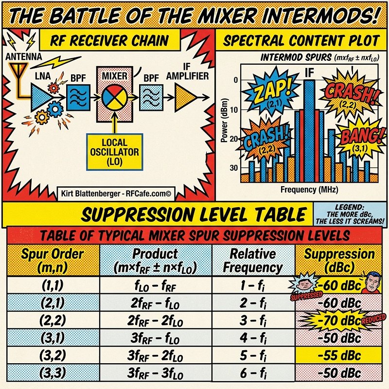
Executive Summary

Spurious frequency intermodulation products, often called mixer spurs, are unwanted output frequencies generated by the nonlinear action of a frequency mixer. In a diode mixer, the same nonlinear diode behavior that makes frequency conversion possible also generates many additional frequencies besides the desired conversion product.

The general mixer spur equation is:

f_SPUR = abs(mf_RF ± nf_LO)

where f_RF is the RF input frequency, f_LO is the local oscillator frequency, and m and n are integer harmonic coefficients. In ordinary frequency conversion, the desired output is usually the 1 x 1 product:

f_IF = abs(1f_RF - 1f_LO)

or, in an upconverter:

f_{RF OUT} = 1f_IF + 1f_LO

All other products, such as 2RF - 1LO, 3RF - 2LO, 1RF + 3LO, 5RF - 4LO, and so forth, are generally undesired unless the mixer is intentionally being used as a harmonic mixer.

Mixer spurs matter because they can fall inside the desired IF, RF output, receiver passband, adjacent channel, image band, ADC Nyquist zone, or regulatory measurement bandwidth. Even a spur that is small at the mixer output can become serious if it is amplified by later gain stages or if it appears inside a sensitive receiver channel.

The practical industry method for estimating mixer spurs is to use a manufacturer-supplied m x n spur suppression table. These tables normally list the suppression, in dBc, of each mRF ± nLO product relative to the desired 1 x 1 output at a specified RF input power, LO drive level, frequency range, and impedance environment. Manufacturer spur tables are empirical and are usually more reliable than purely theoretical hand calculations.

For a first-order estimate at a different RF input level, with LO power held constant and the mixer not compressed, a spur that is m-th order in RF changes approximately m dB for every 1 dB change in RF input power. The desired 1 x 1 output changes approximately 1 dB for every 1 dB change in RF input power. Therefore, the relative suppression of an m x n product changes approximately (m - 1) dB for each 1 dB RF input change.

High-end RF simulators predict mixer intermodulation products using harmonic balance, periodic steady-state methods, transient simulation with FFT, Volterra-series methods, X-parameters, or behavioral spur-table models. Circuit-level tools solve nonlinear diode equations directly; system-level tools often use measured spur tables combined with gain, filtering, compression, IP2, IP3, noise, and impedance models.

Key Findings

• Diode mixers create spurious intermodulation products because their current-versus-voltage characteristic is nonlinear.
• The general mixer spur equation is f_SPUR = abs(mf_RF ± nf_LO).
• The desired frequency conversion product is usually the 1 x 1 product. Other m x n products must be treated as potential spurs.
• Single-ended mixers have the richest spur spectrum because they provide little inherent cancellation.
• Single-balanced mixers suppress some products associated with the balanced port.
• Double-balanced mixers suppress LO feedthrough, RF feedthrough, and many even-order products, but real devices still produce residual spurs.
• Triple-balanced mixers generally provide better isolation, wider bandwidth, higher linearity, and improved spur suppression, but require more LO power and cost more.
• Manufacturer spur tables are the standard practical tool for estimating m x n mixer spur levels.
• Spur suppression is commonly given in dBc relative to the desired 1 x 1 converted output, not as an absolute power.
• RF-level scaling is often approximated by P_SPUR,new = P_SPUR,old + m*(P_RF,new - P_RF,old).
• This scaling rule is approximate and can fail near compression, with incorrect LO drive, with poor port terminations, or when the spur is dominated by leakage or imbalance rather than nonlinear order.
• LO drive level, IP2, IP3, conversion loss, compression point, isolation, and VSWR all affect mixer spur performance.
• Image response, half-IF spurs, 2IF products, LO harmonics, RF harmonics, and ADC aliasing are common frequency-planning traps.
• Laboratory verification is essential for high-performance receivers and transmitters because mixer spur behavior depends strongly on the actual impedance environment.

Detailed Analysis

1. Definition of Spurious Frequency Intermodulation Products

A mixer is a nonlinear device used to translate signals from one frequency to another. In an ideal mathematical multiplier, an RF signal and LO signal produce only the sum and difference frequencies:

f_SUM = f_RF + f_LO
f_DIFFERENCE = abs(f_RF - f_LO)

A real diode mixer is not an ideal multiplier. It produces a larger family of products:

f_SPUR = abs(mf_RF ± nf_LO)

where m and n are integers such as 0, 1, 2, 3, and so forth. Mixer data sheets and system spur charts commonly evaluate m and n from 0 through 10. Products are usually named by their coefficients. For example:

1 x 1 means 1RF ± 1LO.
2 x 1 means 2RF ± 1LO.
3 x 2 means 3RF ± 2LO.
0 x 1 means LO feedthrough or an LO harmonic with no RF contribution.
1 x 0 means RF feedthrough or an RF harmonic with no LO contribution.

In most heterodyne systems, the desired product is the 1 x 1 product. The 1 x  1 difference product is normally the IF in a downconverter. The 1 x 1 sum or difference product may be the desired RF output in an upconverter.

Industry references that discuss these definitions include Mini-Circuits mixer application note AN00-010, Mini-Circuits mixer FAQ material, Marki Microwave mixer basics primer, and Analog Devices MT-080, Mixers and Modulators.

2. Cause of Spurious Products in Diode Mixers

A diode has a nonlinear current-voltage relationship. A simplified diode equation is:

i = I_S*(exp(v/(nV_T)) - 1)

For analysis, the diode current can be approximated as a power series:

i = a₀ + a₁v + a₂v² + a₃v³ + a₄v⁴ + …

If the voltage applied to the diode contains both RF and LO components:

v = Acos(2pif_RFt) + Bcos(2pi*f_LO*t)

then the squared, cubed, and higher-power terms generate sums and differences of the RF and LO frequencies. For example, the v² term can produce f_RF + f_LO and f_RF - f_LO. The v³ term can produce 2f_RF ± f_LO, 2f_LO ± f_RF, 3f_RF, and 3f_LO. Higher-order terms produce still more combinations.

A diode ring mixer is often analyzed as a switching mixer. The LO drives the diode ring so that the RF signal is multiplied by an approximate square-wave switching function. A square wave contains harmonics, so the RF signal can be translated not only by f_LO, but also by LO harmonics such as 3f_LO, 5f_LO, and 7f_LO. In an ideal double-balanced switching mixer, symmetry cancels many unwanted components. In a real mixer, diode mismatch, transformer imbalance, junction capacitance, finite LO drive, parasitic coupling, and imperfect terminations allow residual spurs to appear.

3. How Spurs Affect RF System Performance

Mixer spurs affect both spectral purity and receiver or transmitter performance.

4. The Standard Spur-Frequency Calculation

The standard calculation is simple in frequency and difficult in amplitude.

Frequency Calculation:

For every m and n of interest, calculate:

f_SPUR = abs(mf_RF + nf_LO)
f_SPUR = abs(mf_RF - nf_LO)

Then compare each result to every sensitive frequency range in the system, including IF filters, RF filters, image bands, ADC input bandwidth, Nyquist zones, second-conversion IFs, and transmitter output masks.

Amplitude Calculation:

The amplitude of each product is usually estimated from measured manufacturer spur tables or from nonlinear circuit simulation. Pure hand calculation is rarely accurate enough because real amplitude depends on diode I-V behavior, LO drive, diode matching, balun balance, frequency, port impedances, parasitic capacitance, and package layout.

5. Standard Method of Measuring Mixer Spurious Products

Mixer spurs are measured by applying known RF and LO signals to the mixer and measuring the desired output and unwanted products with a calibrated spectrum analyzer or receiver.

A typical downconverter test setup is:

LO source -> LO filter -> attenuator or pad -> mixer LO port
RF source -> RF filter -> attenuator or pad -> mixer RF port
Mixer IF port -> IF filter or broadband pad -> spectrum analyzer

A typical upconverter test setup is:

LO source -> LO filter -> attenuator or pad -> mixer LO port
IF source -> IF filter -> attenuator or pad -> mixer IF port
Mixer RF port -> RF filter or pad -> spectrum analyzer

Measurement Procedure:

1. Set the LO drive to the manufacturer-specified level, such as +7 dBm, +10 dBm, +13 dBm, +17 dBm, or +23 dBm.
2. Set the RF input power to the level used for the spur table, commonly -10 dBm, although this varies by manufacturer and mixer class.
3. Measure the desired 1 x 1 converted output power.
4. Calculate conversion loss: conversion loss = P_{RF input} - P_{IF desired output}.
5. Tune the analyzer to each expected m x n product frequency.
6. Measure each product power.
7. Express suppression as dBc relative to the desired 1 x 1 output: suppression = P_{desired output} - P_spur.
8. Correct for cable loss, pad loss, analyzer input attenuation, filter loss, and any external gain.
9. Repeat across the relevant RF, LO, and IF frequency range.

Measurement Precautions:

• The RF and LO sources must have low harmonic and spurious content, or they must be filtered.
• The spectrum analyzer must not be overloaded, or it will generate its own intermodulation products.
• Pads and isolators are often used to improve port match and measurement repeatability.
• The analyzer noise floor must be well below the measured spur.
• The measured spur should be checked by changing RF input power. An m-th-order RF spur should move approximately m dB for each 1 dB RF input change.
• LO drive must be held constant when using ordinary RF-order scaling rules.
• Port terminations matter. A mixer measured with broadband 50-ohm pads may not behave identically in the final circuit.

6. Mixer Electrical Parameters That Affect Spurs

7. LO Drive and Mixer Level

Passive diode mixers are often classified by LO drive level. A Level 7 mixer nominally uses about +7 dBm LO drive. Higher-level mixers may use +10 dBm, +13 dBm, +17 dBm, +23 dBm, or more.

Higher LO drive generally gives:

• Higher compression point.
• Higher IP3.
• Better large-signal handling.
• Often improved spur performance for strong RF signals.
• More LO power consumption and more demanding LO chain design.

Underdriving a diode mixer is a common error. If the LO drive is too low, the diodes do not switch cleanly. Conversion loss may increase, isolation may degrade, and spur levels may worsen. Overdriving can also be harmful if it exceeds ratings or creates excessive LO leakage and harmonics.

8. IP2 and IP3 in Relation to Mixer Spurs

IP2 describes second-order distortion. In an ideal double-balanced mixer, even-order products cancel. In a real mixer, imbalance allows even-order products to remain. IP2 is especially important for:

• Half-IF spurs.
• Direct-conversion receiver DC offsets.
• Second-order blocker products.
• Products involving 2RF, 2LO, or 2IF.

IP3 describes third-order distortion. For two RF tones f₁ and f₂, third-order products occur at:

2f₁ - f₂
2f₂ - f₁

In a mixer, these products are translated by the LO and may appear around the IF. If each input tone is at P_IN and the mixer input third-order intercept is IIP3, the approximate spacing between the desired output tone and third-order intermodulation product is:

Delta = 2*(IIP3 - P_IN)

For a passive mixer:

OIP3 Approximately Equals IIP3 - Conversion Loss

IP3 is not the same as a single-tone m x n spur table. IP3 describes two-tone intermodulation. A spur table describes products between a single RF tone and the LO harmonics. Both are needed in serious RF system design.

9. VSWR, Terminations, and Why Mixer Ports are Troublesome

Mixers are not ordinary 50-ohm linear components. They generate energy at many frequencies. If unwanted frequencies are reflected back into the mixer, they can remix and create new in-band products.

For example:

Mixer creates 2RF product -> 2RF product reflects from IF or RF filter -> reflected signal re-enters mixer -> reflected signal mixes with LO harmonic -> new product falls into IF.

This is why a mixer that looks good in a manufacturer test fixture can behave differently in a real receiver. Practical methods to control this include:

• Use attenuator pads where noise figure and gain budget allow.
• Use diplexers at the IF port so out-of-band mixer products see a broadband termination.
• Filter LO harmonics before the mixer LO port.
• Avoid placing a narrowband reflective filter directly on a mixer port unless the out-of-band impedance is controlled.
• Use isolators or buffer amplifiers at microwave frequencies when practical.
• Evaluate mixer behavior with the actual surrounding filters and amplifiers.

10. Single-Ended, Single-Balanced, Double-Balanced, and Triple-Balanced Mixers

Single-Ended Diode Mixer

A single-ended mixer may use a single diode or one nonlinear junction with RF and LO applied simultaneously. It has little symmetry, so almost all m x n products are possible.

Single-Balanced Diode Mixer

A single-balanced mixer uses two nonlinear devices and a transformer, balun, or hybrid so that one port is balanced. Depending on the topology, it can suppress LO feedthrough or RF feedthrough and cancel some even-order products.

Double-Balanced Diode Mixer

The classic double-balanced mixer uses a four-diode ring and baluns or transformers. It is one of the most widely used RF mixer types. In an ideal double-balanced mixer, RF and LO feedthrough are canceled, and many even-order products are suppressed. In real mixers, imperfections limit cancellation.

Triple-Balanced Diode Mixer

A triple-balanced mixer uses more elaborate diode and balun structures to improve balance and isolation over broad bandwidths. Marki Microwave and other microwave mixer manufacturers discuss these tradeoffs in their mixer application literature, including Marki Microwave technical resources.

11. The standard manufacturer spur table method

A manufacturer spur table lists the suppression of mRF ± nLO products relative to the desired 1 x 1 output. The suppression is usually stated in dBc. A value of 60 dBc means the spur is 60 dB below the desired converted output.

A table is valid only under its stated conditions, which commonly include:

• RF input power.
• LO drive power.
• RF frequency.
• LO frequency.
• IF frequency.
• Temperature.
• Source and load impedance.
• Measurement bandwidth and test setup.

Mini-Circuits, Marki Microwave, Analog Devices, Qorvo, and other RF component manufacturers commonly provide mixer specifications, intermodulation data, or application notes explaining the use of such data. See Mini-Circuits AN00-010, Mini-Circuits mixer FAQs, Marki Microwave mixer basics primer, and Analog Devices MT-080.

12. Example Spur Table 1: Representative Double-Balanced Mixer Table

The following is a representative example for explaining the method. It is not a data sheet for a specific mixer. In a real design, use the actual table supplied by the mixer manufacturer.

Assumed test conditions:

RF input power = -10 dBm
LO drive = +7 dBm
Conversion loss = 7 dB
Desired 1 x 1 IF output = -17 dBm
Table entries = suppression in dBc relative to desired 1 x 1 IF output
Rows = m coefficient of RF
Columns = n coefficient of LO

13. How to Use Spur Table 1 to Calculate Absolute Spur Power

Assume:

f_RF = 1000 MHz
f_LO = 900 MHz
Desired IF = abs(1000 - 900) = 100 MHz
RF input power = -10 dBm
Conversion loss = 7 dB
Desired IF output = -17 dBm

From the table, the 3 x 2 product has suppression of 65 dBc.

The possible 3 x 2 frequencies are:

3RF - 2LO = 31000 - 2900 = 3000 - 1800 = 1200 MHz
3RF + 2LO = 31000 + 2900 = 3000 + 1800 = 4800 MHz

The absolute 3 x 2 spur power is:

P_SPUR = P_{desired IF} - suppression

P_SPUR = -17 dBm - 65 dB = -82 dBm

So, under the table conditions, the 3RF - 2LO product at 1200 MHz and the 3RF + 2LO product at 4800 MHz are estimated at approximately -82 dBm before external filtering. In a real manufacturer table, plus and minus products may be listed separately or may differ somewhat; if only one suppression value is given, treat it as an estimate.

14. Using RF-Level Scaling with Spur Table 1

The standard approximate RF-level scaling rule is:

P_SPUR,new = P_SPUR,table + m*(P_RF,new - P_RF,table)

The desired 1 x 1 output scales approximately as:

P_IF,new = P_IF,table + 1*(P_RF,new - P_RF,table)

The new suppression relative to the desired output is:

Suppression_new = Suppression_table - (m - 1)*(P_RF,new - P_RF,table)

Example A: RF input reduced from -10 dBm to -20 dBm.

RF change = -20 - (-10) = -10 dB
m = 3 for a 3 x 2 product
Original 3 x  2 spur = -82 dBm
Original desired IF = -17 dBm

New desired IF:

-17 + 1*(-10) = -27 dBm

New 3 x 2 spur:

-82 + 3*(-10) = -112 dBm

New suppression:

-27 - (-112) = 85 dBc

or:

65 - (3 - 1)*(-10) = 65 + 20 = 85 dBc

Reducing the RF input by 10 dB improves this third-order spur by 20 dB relative to the desired 1 x 1 output.

Example B: RF input increased from -10 dBm to 0 dBm.

RF change = 0 - (-10) = +10 dB
m = 3
Original 3 x 2 spur = -82 dBm
Original desired IF = -17 dBm

New desired IF, if not compressed:

-17 + 10 = -7 dBm

New 3 x 2 spur:

-82 + 3*10 = -52 dBm

New suppression:

-7 - (-52) = 45 dBc

or:

65 - (3 - 1)*10 = 45 dBc

The spur became 30 dB stronger in absolute power and 20 dB worse relative to the desired converted output. This example also shows why the calculation must be checked against the mixer compression point. A Level 7 mixer may not remain linear with 0 dBm RF input in every application.

15. Example Spur Table 2: Representative High-Level Triple-Balanced Mixer Table

The following representative table illustrates how a higher-level, better-balanced mixer may show improved suppression. It is not a substitute for an actual data sheet.

Assumed test conditions:

RF input power = -10 dBm
LO drive = +17 dBm
Conversion loss = 8 dB
Desired 1 x 1 IF output = -18 dBm
Table entries = suppression in dBc relative to desired 1 x 1 output

16. How to Use Spur Table 2 for a Half-IF Spur Estimate

Half-IF spurs are a common receiver problem. Suppose:

LO frequency = 900 MHz
Desired IF = 100 MHz
Desired RF = 1000 MHz, using low-side LO injection

A strong interfering signal at:

f_INT = f_LO + f_IF/2 = 900 + 50 = 950 MHz

can create an IF output through the 2 x 2 product:

2f_INT - 2f_LO = 2950 - 2900 = 1900 - 1800 = 100 MHz

That is exactly the desired IF. From table 2, the 2 x 2 suppression is 78 dBc at RF input = -10 dBm and LO = +17 dBm.

Assume the interfering signal at the mixer RF port is -10 dBm. The desired 1 x 1 output level corresponding to a -10 dBm RF input and 8 dB conversion loss is:

P_1x1 = -10 dBm - 8 dB = -18 dBm

The estimated half-IF spur power is:

P_2x2 = -18 dBm - 78 dB = -96 dBm

If the interfering signal is instead 0 dBm at the mixer input, and the mixer remains outside compression, the 2 x 2 spur changes with m = 2:

RF change = 0 - (-10) = +10 dB
New desired 1 x 1 reference output = -18 + 10 = -8 dBm
New 2 x 2 spur absolute power = -96 + 2*10 = -76 dBm
New suppression = -8 - (-76) = 68 dBc

or:

Suppression_new = 78 - (2 - 1)*10 = 68 dBc

This illustrates why half-IF performance is often dominated by strong blockers. A second-order spur gets 20 dB stronger for a 10 dB blocker increase, while the desired 1 x 1 reference changes only 10 dB.

17. Example of frequency-plan table for a 1000 MHz RF and 900 MHz LO

Assume f_RF = 1000 MHz and f_LO = 900 MHz. The desired IF is 100 MHz. The following table lists selected products. It is not a suppression table; it is a frequency table.

This table shows why high-order products cannot be ignored automatically. The 8 x 9 product may be weak, but it lands exactly on the 100 MHz IF. If the RF signal is strong enough, or if the desired receiver sensitivity is very high, even high-order products may need to be included in the spur budget.

18. Image Frequency

The image frequency is not normally a nonlinear intermodulation product. It is an unwanted 1 x 1 conversion response. It is still one of the most important unwanted mixer responses.

For a downconverter:

f_IF = abs(f_RF - f_LO)

There are two RF frequencies that produce the same IF:

f_RF,desired = f_LO + f_IF
f_RF,image = f_LO - f_IF

or the reverse, depending on whether high-side or low-side LO injection is used.

The separation between desired RF and image RF is:

Image Separation = 2*f_IF

Example:

LO = 900 MHz
Desired RF = 1000 MHz
IF = 100 MHz
Image RF = 800 MHz
Image separation = 1000 - 800 = 200 MHz = 2*IF

Low IF makes image filtering difficult because the image is close to the desired RF. High IF improves image rejection but may make IF filtering and ADC sampling more difficult. Image-reject mixers, Hartley receivers, Weaver receivers, and quadrature sampling architectures are common solutions. Their image rejection is limited by amplitude and phase balance.

19. 2IF Concerns

The term 2IF can refer to several related design problems.

20. Other Common Mixer Spur "Gotchas"

LO Feedthrough: The 0 x 1 product is LO leakage. In receivers, LO leakage can radiate from the antenna. In transmitters, LO feedthrough can appear as an unwanted carrier.

RF Feedthrough: The 1 x 0 product is RF leakage. In an upconverter, IF or RF feedthrough may appear at the output if filtering is inadequate.

LO Harmonics: Products such as 0 x 2, 0 x 3, and 0 x 4 may leak through the mixer and appear at output ports.

Odd LO harmonic conversion: In a switching mixer, RF can convert with odd LO harmonics. Products such as 1RF ± 3LO and 1RF ± 5LO can be important in broadband systems.

Subharmonic Responses: Some mixers intentionally use subharmonic LO drive, but unwanted subharmonic responses may appear if LO harmonics or RF harmonics are large.

Reciprocal Conversion: Passive diode mixers are reciprocal to a useful approximation. Signals can enter through ports that were assumed to be outputs and mix in unexpected ways.

Filter Reflection: A filter may reject a spur by reflecting it rather than absorbing it. The reflected spur can remix in the mixer.

LO Phase Noise: LO phase noise is not an m x n spur, but strong blockers can reciprocally mix with LO phase noise and raise the noise floor around the IF.

ADC Aliasing: A spur that is outside the analog IF filter but inside the ADC input bandwidth can alias into the channel after sampling.

Multiple conversion chains: A spur harmless after the first mixer may become harmful after the second mixer.

21. Upconversion Systems

In an upconverter, the lower-frequency IF or baseband signal is translated to RF. The desired product may be:

f_OUT = f_LO + f_IF

or:

f_OUT = abs(f_LO - f_IF)

Common upconverter spurs include:

• LO feedthrough at the RF output.
• IF feedthrough.
• Unwanted sideband.
• 2LO ± IF.
• LO ± 2IF.
• 3LO ± IF.
• 2IF and 3IF products.
• RF harmonics generated by later amplifiers.
• Mixer spurs amplified by the driver and power amplifier chain.

In a transmitter, a mixer spur may be small at the mixer output but large after 40 dB or 60 dB of gain. Transmitter spur analysis must include post-mixer gain and filtering.

22. Downconversion Systems

In a receiver downconverter, the mixer translates an RF signal to an IF. Common downconverter concerns include:

• Image response.
• Half-IF response.
• Strong out-of-band blockers creating in-band products.
• LO leakage back toward the antenna.
• RF leakage into the IF chain.
• IF feedthrough in multi-conversion systems.
• LO harmonic mixing with RF signals.
• Intermodulation between multiple RF signals.
• Reciprocal mixing caused by LO phase noise.

The front-end preselector and mixer are inseparable in this analysis. A high-linearity mixer cannot save a receiver if the preselector allows very strong signals at known spur-producing frequencies.

23. Historical Development of Mixer Spur Analysis

The exact origin of the modern 0-through-10 m x n mixer spur table is uncertain. It appears to have developed as an engineering practice among microwave receiver designers, mixer manufacturers, radar engineers, and test-equipment companies rather than from one single inventor.

Important people, organizations, and places include:

• Edwin H. Armstrong, working in the United States, developed the superheterodyne receiver architecture during the World War I era. The superheterodyne receiver made mixer images, LO leakage, and spurious frequency conversion central design problems. See Encyclopaedia Britannica on Edwin Armstrong.
• Bell Telephone Laboratories, especially in New Jersey, contributed heavily to receiver theory, microwave systems, and practical communication engineering. Harald T. Friis is best known for noise and cascade analysis, but the same system-level thinking underlies spur budgeting. See Bell Labs historical material on Friis.
• Watkins-Johnson Company, historically associated with Palo Alto and San Jose, California, published influential receiver and microwave application notes that helped popularize practical spur charts and frequency-planning methods.
• Stephen A. Maas made major contributions to nonlinear microwave circuit and mixer analysis. His books Microwave Mixers and Nonlinear Microwave and RF Circuits, published by Artech House, are standard references.
• William F. Egan wrote important RF system-design references including Practical RF System Design, covering intercept points, frequency planning, and spurious response analysis.
• Hewlett-Packard, later Agilent and Keysight, helped develop practical RF and microwave measurement methods and harmonic-balance simulation tools. See Keysight Technologies.
• Compact Software, EEsof, Agilent ADS, AWR, Cadence, and Ansys helped commercialize nonlinear RF simulation methods used to calculate mixer products.

24. How High-End RF Simulators Calculate Mixer IMD

Harmonic Balance

Harmonic balance is the most common frequency-domain method for nonlinear RF and microwave circuits. It assumes the circuit reaches a steady state containing many harmonics and mixing products. Linear networks are solved in the frequency domain, while nonlinear elements such as diodes are evaluated using their nonlinear current-voltage equations. The simulator iterates until voltages and currents are consistent.

The output includes amplitudes at frequencies such as:

f_RF ± f_LO
2f_RF ± f_LO
f_RF ± 2f_LO
3f_RF ± 2f_LO
mf_RF ± nf_LO

Commercial tools using harmonic-balance methods include Keysight PathWave ADS, Cadence AWR Design Environment, and other microwave CAD platforms.

Periodic Steady-State Methods

Periodic steady-state, or PSS, methods solve the nonlinear circuit around a large periodic LO drive. Once the LO-driven operating state is found, the simulator can calculate conversion gain, noise, small-signal transfer, and distortion around that state. Cadence SpectreRF is a well-known commercial implementation of this style of RF analysis.

Transient Simulation Plus FFT

A time-domain simulator can apply RF and LO signals, calculate the waveform, and use an FFT to find spurs. This is conceptually simple but can be slow and requires careful frequency planning, time step control, windowing, and simulation length.

Volterra-Series Analysis

Volterra methods model weak nonlinearities using nonlinear kernels. They are useful for insight and for mildly nonlinear circuits. They are less convenient for strongly switched diode mixers because the LO drive is large and the circuit is highly time-varying.

X-parameters and Nonlinear Behavioral Models

X-parameters extend S-parameter concepts to nonlinear RF devices under large-signal excitation. They can model harmonic generation and mixing behavior around a specified large-signal operating point. Keysight has published application material on this method, including Keysight X-parameter application literature.

Behavioral Spur-Table Models

System-level RF simulators often use behavioral mixer models rather than detailed diode models. These models include conversion loss, noise figure, compression, IP2, IP3, isolation, and an m x n spur table. The simulator computes spur frequencies, applies table suppression values, scales them with signal power, then propagates them through filters, amplifiers, attenuators, ADCs, and later mixers.

This approach is fast and practical for receiver and transmitter architecture studies. Its accuracy depends on the quality of the measured data and whether the real circuit matches the measurement conditions.

25. Practical Spur Suppression Methods

26. Practical Frequency-Planning Workflow

A good mixer spur analysis process is:

1. Define every RF, LO, IF, and output tuning range.
2. Decide which products to evaluate, commonly m and n from 0 through 10.
3. Calculate abs(mf_RF + nf_LO) and abs(mf_RF - nf_LO) across the entire tuning range.
4. Identify products falling inside desired passbands, image bands, IF filters, ADC bandwidths, and protected transmit bands.
5. Use manufacturer spur tables to estimate product levels.
6. Scale spur levels for actual RF input and blocker levels.
7. Include conversion loss, filter rejection, amplifier gain, compression, IP2, IP3, and noise floor.
8. Check image, half-IF, 2IF, LO harmonic, and ADC alias products explicitly.
9. Repeat for worst-case temperature, LO drive tolerance, frequency extremes, and component tolerances.
10. Verify the final design in the lab using clean signal sources and calibrated measurements.

27. Open Questions and Debates in the Field

Measured Tables Versus Simulation

Measured tables are highly valuable because they include real diode imbalance, balun behavior, layout, package parasitics, and practical LO drive. However, they may not cover the exact frequency, power, or impedance environment of the final design. Simulation can explore more cases, but only if the nonlinear models are accurate.

How Reliable are Ideal Balance Rules?

Ideal double-balanced and triple-balanced mixers cancel many products. Real mixers do not have perfect diode matching, balun symmetry, or isolation. Ideal selection rules are useful for intuition but cannot replace measured data.

How High Should m and n Go?

0-through-10 tables are common. Some high-dynamic-range systems need products beyond tenth order, especially when blockers are very strong or when a high-order product falls exactly into the IF.

How Should Out-of-Band Impedances Be Modeled?

Mixer spur levels depend on port impedances not only at RF, LO, and IF, but also at harmonic, image, and spur frequencies. These impedances are often unknown or poorly controlled in practical systems.

Can IP2 and IP3 Replace Spur Tables?

No. IP2 and IP3 are useful large-signal linearity metrics, but they do not uniquely predict every m x n spur. Spur tables, intercept points, compression data, and measurement all describe different parts of mixer behavior.

How do Diode Mixer Rules Apply to Active Mixers?

The same m x n frequency relationships apply to active mixers, CMOS passive FET mixers, and Gilbert-cell mixers. However, the amplitude mechanisms differ. Active mixers include transistor transconductance nonlinearities, switching-pair imbalance, flicker noise, DC offset mechanisms, substrate coupling, and bias-dependent effects.

28. Sources Cited and Recommended References

• Mini-Circuits, mixer application note AN00-010, practical definitions and mixer measurement concepts.
• Mini-Circuits, frequently asked questions about mixers, practical mixer terminology and performance issues.
• Marki Microwave, Mixer Basics Primer, diode mixer concepts, balance, LO drive, and practical selection issues.
• Marki Microwave technical resources, application notes on mixer performance and topology tradeoffs.
• Analog Devices MT-080, Mixers and Modulators, tutorial on mixer and modulator fundamentals.
• Analog Devices technical articles, RF receiver and transmitter architecture material, including image-reject and quadrature concepts.
• Stephen A. Maas, Microwave Mixers, Artech House, major reference on mixer theory and practice.
• Stephen A. Maas, Nonlinear Microwave and RF Circuits, Artech House, major reference on nonlinear RF analysis.
• William F. Egan, Practical RF System Design, Wiley, widely used RF system-design reference for intercept points, spurs, and cascaded analysis.
• David M. Pozar, Microwave Engineering, Wiley, general microwave engineering background.
• Keysight PathWave ADS, commercial RF and microwave simulation platform using harmonic balance and system simulation methods.
• Keysight X-parameters application note, nonlinear RF behavioral modeling.
• Cadence SpectreRF, periodic steady-state and RF circuit simulation methods.
• Cadence AWR RF and microwave design tools, nonlinear and system-level RF design tools.
• Encyclopaedia Britannica, Edwin Howard Armstrong, historical background on the superheterodyne receiver.
• Bell Labs historical material on Harald T. Friis, background on system-level receiver analysis traditions.

29. Final Conclusions

Mixer intermodulation spurious products are unavoidable in diode frequency converters. The designer’s job is to predict where they occur, estimate how large they are, suppress them with balance and filtering, and choose a frequency plan that prevents troublesome products from landing in sensitive bands.

The essential practical tools are:

• The equation f_SPUR = abs(mf_RF ± nf_LO).
• Manufacturer m x n spur tables.
• RF-level scaling based on the m coefficient.
• IP2 and IP3 data.
• Conversion loss and compression data.
• Careful image, half-IF, 2IF, LO harmonic, and ADC alias analysis.
• Proper LO drive and good broadband terminations.
• Nonlinear simulation and laboratory verification.

The most common mistake is to evaluate only the desired 1 x 1 conversion and the image frequency. That is not enough. A robust RF design must examine the full m x n spur environment over all operating frequencies and signal levels. In high-performance receivers and transmitters, mixer spur analysis is a system-level design discipline, not merely a data-sheet lookup.

This content was generated primarily with the assistance of ChatGPT (OpenAI), and/or Gemini (Google), and/or Arya (GabAI), and/or Grok (x.AI), and/or DeepSeek artificial intelligence (AI) engines. Review was performed to help detect and correct any inaccuracies; however, you are encouraged to verify the information yourself if it will be used for critical applications. In all cases, multiple solicitations to the AI engine(s) was(were) used to assimilate final content. Images and external hyperlinks have also been added occasionally - especially on extensive treatises. Courts have ruled that AI-generated content is not subject to copyright restrictions, but since I modify them, everything here is protected by RF Cafe copyright. Many of the images are likewise generated and modified. Your use of this data implies an agreement to hold totally harmless Kirt Blattenberger, RF Cafe, and any and all of its assigns. Thank you. Here is Gab AI in an iFrame.

AI Technical Trustability Update

While working on an update to my RF Cafe Espresso Engineering Workbook project to add a couple calculators about FM sidebands (available soon). The good news is that AI provided excellent VBA code to generate a set of Bessel function plots. The bad news is when I asked for a table showing at which modulation indices sidebands 0 (carrier) through 5 vanish, none of the agents got it right. Some were really bad. The AI agents typically explain their reason and method correctly, then go on to produces bad results. Even after pointing out errors, subsequent results are still wrong. I do a lot of AI work and see this often, even with subscribing to professional versions. I ultimately generated the table myself. There is going to be a lot of inaccurate information out there based on unverified AI queries, so beware.

Electronics & High Tech Companies | Electronics & Tech Publications | Electronics & Tech Pioneers | Electronics & Tech Principles | Tech Standards Groups & Industry Associations | Societal Influences on Technology