Module 12 − Modulation Principles
Pages i,
1−1,
1−11,
1−21,
1−31,
1−41,
1−51,
1−61,
1−71,
2−1,
2−11,
2−21,
2−31,
2−41,
2−51,
2−61,
3−1,
3−11,
3−21,
3−31, AI−1, Index, Assignment 1, 2
one gas tube is
required to discharge the pulse-forming network, and a low amplitude trigger pulse is sufficient to initiate
discharge. a damping diode is used to prevent breakdown of the thyratron by reverse-voltage transients. The
thyratron requires a sharp leading edge for a trigger pulse and depends on a sudden drop in anode voltage
(controlled by the pulse-forming network) to terminate the pulse and cut off the tube. As shown in figure
2-39, the typical thyratron modulator is very similar to the spark-gap modulator. It consists of a power source
(Eb), a circuit for storing energy (L2, C2, C3, C4, and C5), a circuit for discharging the storage circuit (V2),
and a pulse transformer (T1). In addition this circuit has a damping diode (V1) to prevent reverse-polarity
signals from being applied to the plate of V2 which could cause V2 to breakdown. With no trigger pulse
applied, the PFN charges through T1, the PFN, and the charging coil L1 to the potential of Eb. When a trigger
pulse is applied to the grid of V2, the tube ionizes causing the pulse- forming network to discharge through V2
and the primary of T1. As the voltage across the PFN falls below the ionization point of V2, the tube shuts off.
Because of the inductive properties of the PFN, the positive discharge voltage has a tendency to swing negative.
This negative overshoot is prevented from damaging the thyratron and affecting the output of the circuit by V1,
R1, R2, and C1. This is a damping circuit and provides a path for the overshoot transient through V1. It is
dissipated by R1 and R2 with C1 acting as a high-frequency bypass to ground, preserving the sharp leading and
trailing edges of the pulse. The hydrogen thyratron modulator is the most common radar modulator. Pulse modulation
is also useful in communications systems. The intelligence-carrying capability and power requirements for
communications systems differ from those of radar. Therefore, other methods of achieving pulse modulation that are
more suitable for communications systems will now be studied. Q-18. What is the primary component for a
spark-gap modulator? Q-19. What are the basic components of a thyratron modulator?
Communications PULSE ModulatorS To transmit intelligence using pulse modulation, you must provide
a method to vary some characteristic of the pulse train in accordance with the modulating signal. Figure 2-40
illustrates a simple pulse train. The characteristics of these pulses that can be varied are amplitude, pulse
width, pulse-repetition time, and the pulse position as compared to a reference. In addition to these three
characteristics, pulses may be transmitted according to a code to represent the different levels of the modulating
signal. To ensure maximum fidelity (accuracy in reproducing a modulating wave), the modulating signal has to be
represented by enough pulses to restore the original wave shape. Logically, the higher the sampling rate (the more
often sampled) of the pulse modulator, the more accurately the original modulating wave can be reproduced. Figure
2-41 illustrates the effectiveness of three pulse-sampling rates. View (A) shows a sampling rate of more than two
times the modulating frequency. As you can see, this reproduces the modulating signal very accurately. However,
the high sampling rate requires a wide bandwidth and increases the average power required of the transmitter. If
less than two samples per cycle are made, you are not able to reproduce the original modulating signal, as shown
in view (B). View (C) shows a sampling rate that is two times the highest modulating frequency. This is the
minimum sampling rate that will give a sufficiently accurate reproduction of the modulating wave. The standard
sampling rate is 2.5 times the highest frequency that is to be transmitted. This ensures the ability to accurately
reproduce the modulating waveform. In military voice systems the bandwidth for voice signals is limited to 300 to
3,000 hertz, requiring a sampling frequency of 8 kilohertz. Although the pulse characteristic that is changed may
vary for each type of pulse modulation, the sampling frequency will remain constant. We will now briefly discuss
common types of pulse modulation. 2-41
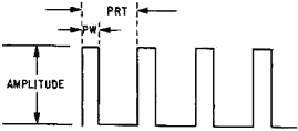
Figure 2-40. - Pulse train.

Figure 2-41A. - Pulse sampling rates. MORE THAN TWO PULSE SAMPLES for EVery WAVE.

Figure 2-41B. - Pulse sampling rates. LESS THAN TWO PULSE SAMPLES for EVery WAVE.
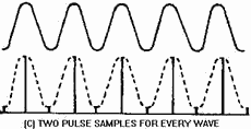
Figure 2-41C. - Pulse sampling rates. TWO PULSE SAMPLES for EVery WAVE.
2-42
Pulse-Amplitude Modulation Some characteristic of the sampling pulses must be varied by the modulating signal for the intelligence of the
signal to be present in the pulsed wave. Figure 2-42 shows three typical waveforms in which the pulse amplitude is
varied by the amplitude of the modulating signal. View (A) represents a sine wave of intelligence to be modulated
on a transmitted carrier wave. View (B) shows the timing pulses which determine the sampling interval. View (C)
shows PULSE-Amplitude MODULATION (PAM) in which the amplitude of each pulse is controlled by the instantaneous
amplitude of the modulating signal at the time of each pulse.

Figure 2-42A. - Pulse-amplitude modulation (PAM). MODULATION.
Figure
2-42B. - Pulse-amplitude modulation (PAM). TIMING.

Figure 2-42C. - Pulse-amplitude modulation (PAM). PAM.
Pulse-amplitude modulation is the simplest form of pulse modulation. It is generated in much the same manner
as analog-amplitude modulation. The timing pulses are applied to a pulse amplifier in which the gain is controlled
by the modulating waveform. Since these variations in amplitude actually represent the signal, this type of
modulation is basically a form of AM. The only difference is that the signal is now in the form of pulses. This
means that PAM has the same built-in weaknesses as any other AM signal - high susceptibility to noise and
interference. The reason for susceptibility to noise is that any interference in the transmission path will either
add to or subtract from any voltage already in the circuit (signal voltage). Thus, the amplitude of the signal
will be changed. Since the amplitude of the voltage represents the signal, any unwanted change to the signal is
considered a Signal Distortion. For this reason, PAM is not often used. When PAM is used, the pulse train is used
to frequency modulate a carrier for transmission. Techniques of pulse modulation other than PAM have been
developed to overcome problems of noise interference. The following sections will discuss other types of pulse
modulation. Q-20. What action is necessary to impress intelligence on the pulse train in pulse
modulation? 2-43
Q-21. To ensure the accuracy of a transmission, what is the minimum number of times a modulating wave should
be sampled in pulse modulation? Q-22. What, if any, noise susceptibility advantage exists for
pulse-amplitude modulation over analog- amplitude modulation? Pulse-Time Modulation
In pulse-modulated systems, as in an analog system, the intelligence may be impressed on the carrier by varying
any of its characteristics. In the preceding paragraphs the method of modulating a pulse train by varying its
amplitude was discussed. Time characteristics of pulses may also be modulated with intelligence information. Two
time characteristics may be affected: (1) the time duration of the pulses, referred to as PULSE-DURATION
MODULATION (PDM) or PULSE-WIDTH MODULATION (pwm); and (2) the time of occurrence of the pulses, referred to as
PULSE-POSITION MODULATION (PPM), and a special type of PULSE-TIME MODULATION (PTM) referred to as PULSE-Frequency
MODULATION (PFM). Figure 2-43 shows these types of PTM in views (C), (D), and (E). Views (A) and (B) show the
modulating signal and timing, respectively.
Figure 2-43A. - Pulse-time modulation (PTM). MODULATION.
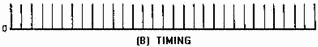
Figure 2-43B. - Pulse-time modulation (PTM). TIMING. 
Figure 2-43C. - Pulse-time modulation (PTM). PDM. 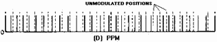
Figure 2-43D. - Pulse-time modulation (PTM). PPM.
2-44

Figure 2-43E. - Pulse-time modulation (PTM). PFM PULSE-DURATION MODULATION. - PDM and PWM are designations for a single type of
modulation. The width of each pulse in a train is made proportional to the instantaneous value of the modulating
signal at the instant of the pulse. Either the leading edges, the trailing edges, or both edges of the pulses may
be modulated to produce the variation in pulse width. PDM can be obtained in a number of ways, one of which is
illustrated in views (A) through (D) in figure 2-44. a circuit to produce PDM is shown in figure 2-45. Adding the
modulating signal [figure 2-44, view (A)] to a repetitive sawtooth [view (B)] will result in the waveform shown in
view (C). This waveform is then applied to a circuit which changes state when the input signal exceeds a specific
threshold level. This action produces pulses with widths that are determined by the length of time that the input
waveform exceeds the threshold level. The resulting waveform is shown in view (D).

Figure 2-44A. - Pulse-duration modulation (PDM). MODULATING Signal.

Figure 2-44B. - Pulse-duration modulation (PDM). REPETITIVE SAWTOOTH PULSES.

Figure 2-44C. - Pulse-duration modulation (PDM). MODULATING Signal and SAWTOOTH ADDED. 2-45
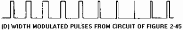
Figure 2-44D. - Pulse-duration modulation (PDM).
WIDTH MODULATED PULSES FROM Circuit of FIGURE 2-45.
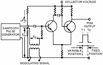
Figure 2-45. - Circuit for producing PDM.
In the circuit of figure 2-45, a series of sawtooth pulses, occurring at the sampling rate, is applied to a
one-shot multivibrator. The multivibrator has the signal voltage Es superimposed on the bias voltage Ein. Each
pulse triggers a cycle of multivibrator operation which terminates after a time interval and varies linearly with
the voltage Es. The pulse of plate voltage produced by the multivibrator will have a leading edge at T1. The
leading edge will vary in position with the signal voltage, while the trailing edge at T2 is fixed by the
termination of the sawtooth pulse. The length of the output pulse is thus duration or width modulated. If the
sawtooth has an instantaneous buildup and a sloping trailing edge, then the leading edge (T1) is fixed and the
trailing edge (T2) varies. If the sawtooth generator produces a slope on both leading and trailing edges, both T1
and T2 are variable in position, but the result is still PDM. PDM is often used because it is of a constant
amplitude and is, therefore, less susceptible to noise. When compared with PPM, PDM has the disadvantage of a
varying pulse, width and, therefore, of varying power content. This means that the transmitter must be powerful
enough to handle the maximum-width pulses, although the average power transmitted is much less than peak power. On
the other hand, PDM will still work if the synchronization between the transmitter and receiver fails; in PPM it
will not, as will be seen in the next section. PULSE-POSITION MODULATION. - The amplitude
and width of the pulse is kept constant in the system. The position of each pulse, in relation to the position of
a recurrent reference pulse, is varied by each instantaneous sampled value of the modulating wave. PPM has the
advantage of requiring constant transmitter power since the pulses are of constant amplitude and duration. It is
widely used but has the disadvantage of depending on transmitter-receiver synchronization. 2-46
PPM can be generated in several ways, but we will discuss one of the simplest. Figure 2-46 shows three
waveforms associated with developing PPM from PDM. The PDM pulse train is applied to a differentiating circuit.
(Differentiation was presented in NEETS, Module 9, Introduction to Wave-Generation and Wave-Shaping Circuits.)
This provides positive- and negative-polarity pulses that correspond to the leading and trailing edges of the PDM
pulses. Considering PDM and its generation, you can see that each pulse has a leading and trailing edge. In this
case the position of the leading edge is fixed, whereas the trailing edge is not, as shown in view (A) of figure
2-46. The resultant pulses after the differentiation are shown in view (B). The negative pulses are
position-modulated in accordance with the modulating waveform. Both the negative and positive pulse are then
applied to a rectification circuit. This application eliminates the positive, non-modulated pulses and develops a
PPM pulse train, as shown in view (C).

Figure 2-46. - Pulse-position modulation (PPM). PULSE-Frequency MODULATION. - PFM is a method of pulse modulation in which the
modulating wave is used to frequency modulate a pulse-generating circuit. For example, the pulse rate may be 8,000
pulses per second (PPS) when the signal voltage is 0. The pulse rate may step up to 9,000 PPS for maximum positive
signal voltage, and down to 7,000 PPS for maximum negative signal voltage. Figure 2-47, views (A), (B), and (C)
show three typical waveforms for PFM. This method of modulation is not used extensively because of complicated PFM
generation methods. It requires a stable oscillator that is frequency modulated to drive a pulse generator. Since
the other forms of PTM are easier to achieve, they are commonly used.

Figure 2-47A. - Pulse-frequency modulation (PFM). MODULATION. 2-47

Figure 2-47B. - Pulse-frequency modulation (PFM). TIMING. 
Figure
2-47C. - Pulse-frequency modulation (PFM). PFM. Q-23. What characteristics of a pulse can be changed in pulse-time modulation? Q-24. Which
edges of the pulse can be modulated in pulse-duration modulation? Q-25. What is the main disadvantage of
pulse-position modulation? Q-26. What is pulse-frequency modulation? Pulse-Code
Modulation PULSE-Code MODULATION (PCM) refers to a system in which the standard values of a QUANTIZED
WAVE (explained in the following paragraphs) are indicated by a series of coded pulses. When these pulses are
decoded, they indicate the standard values of the original quantized wave. These codes may be binary, in which the
symbol for each quantized element will consist of pulses and spaces: ternary, where the code for each element
consists of any one of three distinct kinds of values (such as positive pulses, negative pulses, and spaces); or
n-ary, in which the code for each element consists of nay number (n) of distinct values. This discussion will be
based on the binary PCM system. All of the pulse-modulation systems discussed previously provide methods
of converting analog wave shapes to digital wave shapes (pulses occurring at discrete intervals, some
characteristic of which is varied as a continuous function of the analog wave). The entire range of amplitude
(frequency or phase) values of the analog wave can be arbitrarily divided into a series of standard values. Each
pulse of a pulse train [figure 2-48, view (B)] takes the standard value nearest its actual value when modulated.
The modulating wave can be faithfully reproduced, as shown in views (C) and (D). The amplitude range has been
divided into 5 standard values in view (C). Each pulse is given whatever standard value is nearest its actual
instantaneous value. In view (D), the same amplitude range has been divided into 10 standard levels. The curve of
view (D) is a much closer approximation of the modulating wave, view (A), than is the 5-level quantized curve in
view (C). From this you should see that the greater the number of standard levels used, the more closely the
quantized wave approximates the original. This is also made evident by the fact that an infinite number of
standard levels exactly duplicates the conditions of nonquantization (the original analog waveform). 2-48

Figure 2-48A. - Quantization levels. MODULATION. 
Figure
2-48B. - Quantization levels. TIMING. 
Figure
2-48C. - Quantization levels. QUANTIZED 5-LEVEL. 
Figure
2-48D. - Quantization levels. QUANTIZED 10-LEVEL. Although the quantization curves of figure 2-48 are based on 5- and 10-level quantization, in actual
practice the levels are usually established at some exponential value of 2, such as 4(22), 8(23), 16(24),
32(25) . . . N(2n). The reason for selecting levels at exponential values of 2 will become evident in the
discussion of PCM. Quantized fm is similar in every way to quantized AM. That is, the range of frequency deviation
is divided into a finite number of standard values of deviation. Each sampling pulse results in a deviation equal
to the standard value nearest the actual deviation at the sampling instant. Similarly, for phase modulation,
quantization establishes a set of standard values. Quantization is used mostly in amplitude- and
frequency-modulated pulse systems. Figure 2-49 shows the relationship between decimal numbers, binary
numbers, and a pulse-code waveform that represents the numbers. The table is for a 16-level code; that is, 16
standard values of a quantized wave could be represented by these pulse groups. Only the presence or absence of
the pulses are important. The next step up would be a 32-level code, with each decimal number represented by a
series of five binary digits, rather than the four digits of figure 2-49. Six-digit groups would provide a
64-level code, seven digits a 128-level code, and so forth. Figure 2-50 shows the application of pulse-coded
groups to the standard values of a quantized wave. 2-49
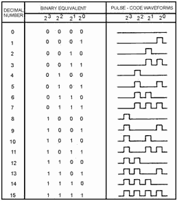
Figure 2-49. - Binary numbers and pulse-code equivalents. 
Figure 2-50. - Pulse-code modulation of a quantized wave (128 bits). In figure 2-50 the solid curve represents the unquantized values of a modulating sinusoid. The dashed
curve is reconstructed from the quantized values taken at the sampling interval and shows a very close agreement
with the original curve. Figure 2-51 is identical to figure 2-50 except that the sampling interval is four times
as great and the reconstructed curve is not faithful to the original. As previously stated, the sampling rate of a
pulsed system must be at least twice the highest modulating frequency to get 2-50
| - |
Matter, Energy,
and Direct Current |
| - |
Alternating Current and Transformers |
| - |
Circuit Protection, Control, and Measurement |
| - |
Electrical Conductors, Wiring Techniques,
and Schematic Reading |
| - |
Generators and Motors |
| - |
Electronic Emission, Tubes, and Power Supplies |
| - |
Solid-State Devices and Power Supplies |
| - |
Amplifiers |
| - |
Wave-Generation and Wave-Shaping Circuits |
| - |
Wave Propagation, Transmission Lines, and
Antennas |
| - |
Microwave Principles |
| - |
Modulation Principles |
| - |
Introduction to Number Systems and Logic Circuits |
| - |
- Introduction to Microelectronics |
| - |
Principles of Synchros, Servos, and Gyros |
| - |
Introduction to Test Equipment |
| - |
Radio-Frequency Communications Principles |
| - |
Radar Principles |
| - |
The Technician's Handbook, Master Glossary |
| - |
Test Methods and Practices |
| - |
Introduction to Digital Computers |
| - |
Magnetic Recording |
| - |
Introduction to Fiber Optics |
| Note: Navy Electricity and Electronics Training
Series (NEETS) content is U.S. Navy property in the public domain. |
|