Module 12 − Modulation Principles
Pages i,
1−1,
1−11,
1−21,
1−31,
1−41,
1−51,
1−61,
1−71,
2−1,
2−11,
2−21,
2−31,
2−41,
2−51,
2−61,
3−1,
3−11,
3−21,
3−31, AI−1, Index, Assignment 1, 2
is referred to as
the MODULATED WAVE and is the waveform that is transmitted through space. When the modulated wave is received and
demodulated, the original component waves (carrier and modulating waves) are reproduced with their respective
frequencies, phases, and amplitudes unchanged. Modulation of a carrier can be achieved by any of several
methods. Generally, the methods are named for the sine-wave characteristic that is altered by the modulation
process. In this module, you will study Amplitude MODULATION, which includes CONTINUOUS-WAVE MODULATION. You will
also learn about two forms of ANGLE MODULATION (Frequency MODULATION and Phase MODULATION). a special type of
modulation, known as PULSE MODULATION, will also be discussed. Before we present the methods involved in
developing modulation, you need to study a process that is essential to the modulation of a carrier, known as
heterodyning. To help you understand the operation of heterodyning circuits, we will begin with a
discussion of LINEAR and NONLINEAR devices. In linear devices, the output rises and falls directly with the input.
In nonlinear devices, the output does not rise and fall directly with the input. LINEAR Impedance Whether the impedance of a device is linear or nonlinear can be determined by comparing the change in current
through the device to the change in voltage applied to the device. The simple circuit shown in view (A) of figure
1-4 is used to explain this process.

Figure 1-4A. - Circuit with one linear impedance. First, the current through the device must be measured as the voltage is varied. Then the current and
voltage values can be plotted on a graph, such as the one shown in view (B), to determine the impedance of the
device. For example, assume the voltage is varied from 0 to 200 volts in 50-volt steps, as shown in view (B). At
the first 50-volt point, the ammeter reads 0.5 ampere. These ordinates are plotted as point a in view (B). With
100 volts applied, the ammeter reads 1 ampere; this value is plotted as point b. As these steps are continued, the
values are plotted as points c and d. These points are connected with a straight line to show the linear
relationship between current and voltage. For every change in voltage applied to the device, a proportional change
occurs in the current through the device. When the change in current is proportional to the change in applied
voltage, the impedance of the device is linear and a straight line is developed in the graph.

Figure 1-4B. - Circuit with one linear impedance. The principle of linear impedance can be extended by connecting two impedance devices in series, as
shown in figure 1-5, view (A). The characteristics of both individual impedances are determined as explained in
the preceding section. For example, assume voltmeter V1 shows 50 volts and the ammeter shows 0.5 ampere. Point a
in view (B) represents this ordinate. In the same manner, increasing the voltage in increments of 50 volts gives
points b, c, and d. Lines Z1 and Z2 show the characteristics of the two impedances. The total voltage of the
series combination can be determined by adding the voltages across Z1 and Z2. For example, at 0.5 ampere, point a
(50 volts) plus point e (75 volts) produces point i (125 volts). Also, at 1 ampere, point b plus point f produces
point j. Line Z1 + Z2 represents the combined voltage-current characteristics of the two devices. 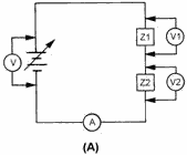
Figure 1-5A. - Circuit with two linear impedances.
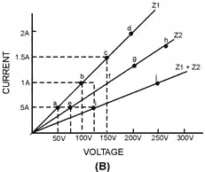
Figure 1-5B. - Circuit with two linear impedances. View (A) of figure 1-6 shows two impedances in parallel. View (B) plots the impedances both individually
(Z1 and Z2) and combined (Z1 x Z2)/(Z1 + Z2). Note that Z1 and Z2 are not equal. At 100 volts, Z1 has 1 ampere of
current plotted at point b and Z2 has 0.5 ampere plotted at point f. The coordinates of the equivalent impedance
of the parallel combination are found by adding the current through Z1 to the current through Z2. For example, at
100 volts, point b is added to point f to determine point j (1.5 amperes).
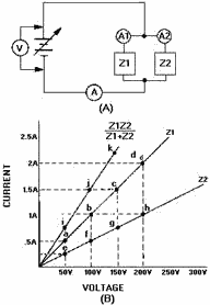
Figure 1-6. - Circuit with parallel linear impedances.
Positive or negative voltage values can be used to plot the voltage-current graph. Figure 1-7 shows an
example of this situation. First, the voltage versus current is plotted with the battery polarity as shown in view
(A). Then the battery polarity is reversed and the remaining voltage versus current points are plotted. As a
result, the line shown in view (C) is obtained. 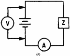
Figure 1-7A. - Linear impedance circuit.
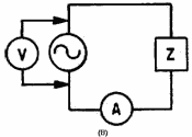
Figure 1-7B. - Linear impedance circuit. 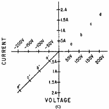
Figure 1-7C. - Linear impedance circuit The battery in view (A) could be replaced with an ac generator, as shown in view (B), to plot the
characteristic chart. The same linear voltage-current chart would result. Current flow in either direction is
directly proportional to the change in voltage. In conclusion, when dc or sine-wave voltages are applied to a
linear impedance, the current through the impedance will vary directly with a change in the voltage. The device
could be a resistor, an air-core inductor, a capacitor, or any other linear device. In other words, if a sine-wave
generator output is applied to a combination of linear impedances, the resultant current will be a sine wave which
is directly proportional to the change in voltage of the generator. The linear impedances do not alter the
waveform of the sine wave. The amplitude of the voltage developed across each linear component may vary, or the
phase of the wave may shift, but the shape of the wave will remain the same.
NONLINEAR Impedance You have studied that a linear impedance is one in which the
resulting current is directly proportional to a change in the applied voltage. a nonlinear impedance is one in
which the resulting current is not directly proportional to the change in the applied voltage. View (A) of figure
1-8 illustrates a circuit which contains a nonlinear impedance (Z), and view (B) shows its voltage-current curve.

Figure 1-8A. - Nonlinear impedance circuit. 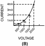
Figure 1-8B. - Nonlinear impedance circuit. As the applied voltage is varied, ammeter readings which correspond with the various voltages can be
recorded. For example, assume that 50 volts yields 0.4 milliampere (point a), 100 volts produces 1 milliampere
(point b), and 150 volts causes 2.2 milliamperes (point c). Current through the nonlinear impedance does not vary
proportionally with the voltage; the chart is not a straight line. Therefore, Z is a nonlinear impedance; that is,
the current through the impedance does not faithfully follow the change in voltage. Various combinations of
voltage and current for this particular nonlinear impedance may be obtained by use of this voltage-current curve.
COMBINED LINEAR and NONLINEAR ImpedanceS The series combination of a linear and a
nonlinear impedance is illustrated in view (A) of figure 1-9. The voltage-current charts of Z1 and Z2 are shown in
view (B). a chart of the combined impedance can be plotted by adding the amount of voltage required to produce a
particular current through linear impedance Z1 to the amount of voltage required to produce the same amount of
current through nonlinear impedance Z2. The total will be the amount of voltage required to produce that
particular current through the series combination. For example, point a (25 volts) is added to point c (50 volts)
which yields point e (75 volts); and point b (50 volts) is added to point d (100 volts) which yields point f (150
volts). Intermediate points may be determined in the same manner and the resultant characteristic curve (Z1 + Z2)
is obtained for the series combination.
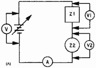
Figure 1-9A. - Combined linear and nonlinear impedances. 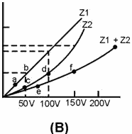
Figure 1-9B. - Combined linear and nonlinear impedances.
You should see from this graphic analysis that when a linear impedance is combined with a nonlinear
impedance, the resulting characteristic curve is nonlinear. Some examples of nonlinear impedances are crystal
diodes, transistors, iron-core transformers, and electron tubes. AC APPLIED to LINEAR and NONLINEAR
ImpedanceS
Figure 1-10 illustrates an ac sine-wave generator applied to a circuit containing several linear impedances. a
sine-wave voltage applied to linear impedances will cause a sine wave of current through them. The wave shape
across each linear impedance will be identical to the applied waveform.

Figure 1-10. - Sine wave generator applied to several impedances. The amplitude, on the other hand, may differ from the amplitude of the applied voltage. Furthermore, the
phase of the voltage developed by any of the impedances may not be identical to the phase of the voltage across
any of the other impedances or the phase of the applied voltage. If an impedance is a reactive component (coil or
capacitor), voltage or current may lead or lag, but the wave shape will remain the same. In a linear circuit, the
output of the generator is not distorted. The frequency remains the same throughout the entire circuit and no new
frequencies are generated. View (A) of figure 1-11 illustrates a circuit that contains a combination of linear
and nonlinear impedances with a sine wave of voltage applied. Impedances Z2, Z3, and Z4 are linear; and Z1 is
nonlinear. The result of a linear and nonlinear combination of impedances is a nonlinear waveform. The curve Z,
shown in view (B), is the nonlinear curve for the circuit of view (A). Because of the nonlinear impedance, current
can flow in the circuit only during the positive alternation of the sine-wave generator. If an oscilloscope is
connected, as shown in view (A), the waveform across Z3 will not be a sine wave. Figure 1-12, view (A),
illustrates the sine wave from the generator and view (B) shows the waveform across the linear impedance Z3.
Notice that the nonlinear impedance Z1 has eliminated the negative half cycles.

Figure 1-11A. - Circuit with nonlinear impedances. 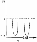
Figure 1-11B. - Circuit with nonlinear impedances. 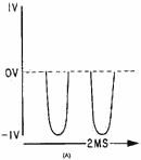
Figure 1-12A. - Waveform in a circuit with nonlinear impedances.

Figure 1-12B. - Waveform in a circuit with nonlinear impedances. The waveform in view (B) is no longer identical to that of view (A) and the nonlinear impedance network
has generated Harmonic FREQUENCIES. The waveform now consists of the fundamental frequency and its harmonics.
(Harmonics were discussed in NEETS, Module 9, Introduction to Wave-Generation and Wave-Shaping Circuits.)
TWO SINE WAVE GENERATORS IN LINEAR Circuits A circuit composed of two sine-wave generators, G1 and
G2, and two linear impedances, Z1 and Z2, is shown in figure 1-13. The voltage applied to Z1 and Z2 will be the
vector sum of the generator voltages. The sum of the individual instantaneous voltages across each impedance
will equal the applied voltages.

Figure 1-13. - Two sine-wave generators with linear impedances.
If the two generator outputs are of the same frequency, then the waveform across Z1 and Z2 will be a sine
wave, as shown in figure 1-14, views (A) and (B). No new frequencies will be created. Relative amplitude and phase
will be determined by the relative values and types of the impedances.
| - |
Matter, Energy,
and Direct Current |
| - |
Alternating Current and Transformers |
| - |
Circuit Protection, Control, and Measurement |
| - |
Electrical Conductors, Wiring Techniques,
and Schematic Reading |
| - |
Generators and Motors |
| - |
Electronic Emission, Tubes, and Power Supplies |
| - |
Solid-State Devices and Power Supplies |
| - |
Amplifiers |
| - |
Wave-Generation and Wave-Shaping Circuits |
| - |
Wave Propagation, Transmission Lines, and
Antennas |
| - |
Microwave Principles |
| - |
Modulation Principles |
| - |
Introduction to Number Systems and Logic Circuits |
| - |
- Introduction to Microelectronics |
| - |
Principles of Synchros, Servos, and Gyros |
| - |
Introduction to Test Equipment |
| - |
Radio-Frequency Communications Principles |
| - |
Radar Principles |
| - |
The Technician's Handbook, Master Glossary |
| - |
Test Methods and Practices |
| - |
Introduction to Digital Computers |
| - |
Magnetic Recording |
| - |
Introduction to Fiber Optics |
| Note: Navy Electricity and Electronics Training
Series (NEETS) content is U.S. Navy property in the public domain. |
|