|
|||||||||||||
 |
|||||||||||||
A Course in Radio Fundamentals - Vacuum Tubes |
|||||||||||||
It's hard for most people alive today to imagine a time when vacuum tubes were the only means of amplification and rectification available. The discovery and application of semiconductors as replacements was a huge step forward for all but the highest power applications like megawatt power amplifiers. Equally hard to imagine is having to design circuits without the aide of computers - or at least a digital calculator. Parameter tables and slide rules were de rigueur for the day. Power supplies in the hundreds of volts were commonplace and printed circuit boards were a platform of the future. Point-to-point wiring ruled the day. Other than for special cases like traveling wave tubes (TWTs) and microwave magnetrons, there are not many engineers left that design tubes. As with a lot of the vintage methods and equipment, it is amateur hobbyists who keep the art of tube circuits alive. The Internet is full of projects and articles on tube design. I have accumulated a few resources over the years right here on RF Cafe. NOTE: References to the Handbook in the Assignments are for the ARRL Handbook of the day. Sorry, I don't have that available. A Course in Radio Fundamentals Lessons in Radio Theory for the Amateur By George Grammer, W1DFNo.4 - Vacuum-Tube Fundamentals
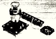
Fig. 1 - Vacuum tube board. Experiments designed to show comprehensively the operation of the vacuum tube as an amplifier require a fairly elaborate array of test apparatus. Finding the gain-frequency characteristic of an audio amplifier, for example, requires the use of a calibrated source of variable frequency over the audio-frequency range, plus a calibrated attenuator and means for measuring voltage with readings independent of frequency, while distortion cannot readily be observed without an oscilloscope. Such equipment is expensive and satisfactory substitutes cannot readily be constructed at home. However, simple experiments designed to show the properties of vacuum tubes readily can be performed with the gear described in the preceding installments. As a convenience in setting up apparatus, a tube board such as is shown in Fig. 1 can be added. It consists simply of a baseboard on which is placed a square piece of Bakelite in which is mounted an ordinary octal socket, connections being brought out from the socket prongs to machine-screw terminals. This permits chanting tube connections without soldering. The heater terminals are permanently connected to a terminal strip mounted at the back of the board; this strip also has terminals for "B" supply, one negative and two positive. The latter take care of separate plate and screen voltages when a tetrode or pentode is used. A push-button mounted on the board provides a means of closing the plate (or screen) circuit when the milliammeter in the test instrument is being used for other measurements. In using the plate power supply with its variable voltage divider it should be remembered that only a limited current can be taken through the divider taps for more than very short periods of time. The variable resistor, in particular, is rated at only a few watts, and if the output current is more than 15 milliamperes or so the time during which current flows must be kept to a minimum. Since a reading can be taken in a mat-ter of seconds this is no handicap, but if the supply is used for continuous output the resistor arm should be set at the end connected to the transformer center tap (see Fig. 4, p. 65, August QST), or else a switch should be provided for shorting between the negative output terminal and the wire connected to the center-tap of the power transformer. Tube Characteristics Some amplification of the Handbook material dealing with tube constants may be helpful in connection with the experimental work. In the paragraph on "Characteristics" (§ 3-2), for instance, plate resistance is defined as "the ratio, for a fixed grid voltage, of a small plate voltage change to the plate current change it effects." This can be written in the form of an equation:
The values of the constants can be found by plotting characteristic curves and measuring the change which occurs in one quantity when the other is changed any arbitrary amount. However, this method must be used with some caution when the characteristic curve does not turn out to be a straight line. If the line bends, the "constant" is not actually always the same, but varies with the point on the curve at which it is measured. For example, suppose that Fig. 2 represents a curve showing the variation of plate current as the plate voltage is varied, and from it we want to determine the plate resistance. We arbitrarily select A as the point from which to start and, also arbitrarily, decide to make the plate current change, Ip 2 milliamperes. A 2-milliampere increase brings us to point B on the curve. Then the corresponding change in plate voltage, Ep, is the difference between the plate voltages which cause 1 and 3 milliamperes to flow. Thus Ep = 70 - 30 = 40 volts. Then
Because of the curvature of the characteristic the value of the "constant" rp as measured by this method will depend considerably upon the value of Δ selected. As the value of Δ is made smaller and smaller the value of the ratio ΔEp/ΔIp approaches the ratio AD/DE, where the line FE is drawn tangent to the curve at point A (that is, the line FE touches but does not intersect the curve at point A). In Fig. 2 this ratio is
which is the value of the plate resistance at point A on the curve. If points B or C had been selected instead of A as the starting place (point at which plate resistance is to be determined) different values of plate resistance would be obtained, since it is obvious that tangents drawn through these points would not coincide with the tangent EF.
Fig. 2 - Basis for measurement of ΔEp and ΔIp chart. In determining the values of the tube constants from the curves, therefore, the preferred procedure is to draw a tangent to the curve at the point at which the value of the constant is to be measured, and then use the tangent line as a basis for measurement of ΔEp and ΔIp (or whatever pair of quantities is represented by the curve). While there is bound to be some inaccuracy in drawing the tangent, in general the results will be nearer the truth than if two points on the curve itself are selected. Of course if the curve is straight the curve and its tangent coincide, so that in the special case of a straight-line curve points can be taken directly from the curve. Caution In the diagrams of the various setups for the experiments to follow, milliammeters and volt-meters are indicated where measurements are to be made. If enough separate instruments are at hand, they may be used as shown. However, if only the single combination test instrument is available for measuring currents and voltages, extreme care should be used to see that the proper range is selected before making voltage measurements. In alternate switching from current to voltage it is only too easy to leave the range switch on 0-1 ma. when connecting the instrument across three or four hundred volts - with consequences easy to imagine. Such an error - bad enough normally - would be practically fatal now, with instrument replacements or repairs virtually impossible. Watch that range switch!
ASSIGNMENT 11 Study Handbook Sections 3-1 and 3-2, starting page 42. Perform Exps. 21, 22 and 23. Questions 1) How does conduction take place in a thermionic vacuum tube? 2) What is the space charge? 3) What is the purpose of the grid in a triode? 4) Name the three fundamental tube characteristics and define them. 5) Why is a "load" necessary if a vacuum tube is to perform useful work? 6) What are tube characteristic curves? 7) Why is amplification possible with a triode tube? 8) What is meant by the term "interelectrode capacity"? 9) What is the difference between static and dynamic characteristic curves? 10) In what form is the power supplied to the plate-cathode circuit of a tube dissipated? 11) What is the purpose of tube ratings? 12) What is meant by the term "plate current cutoff point or"? 13) What is grid bias, and why is it used? 14) Define saturation point. 15) What is rectification?
ASSIGNMENT 12 Study Handbook Sections 3-3 and 3-4, starting page 44. Perform Exp. 24. Questions 1) Name three forms which the plate load for a triode amplifier may take. 2) Define voltage amplification; power amplification. What is the essential difference between amplifiers designed for the two purposes? 3) What determines the choice of operating point for an amplifier? 4) Define plate efficiency. How does it vary with different types of operation (Class A, B and C)? 5) What is harmonic distortion and how is it caused? 6) Describe Class-A amplifier operation. 7) What is feedback? What is the result of application of positive feedback? Of negative feedback? 8) How is the input capacity of a triode amplifier affected by its operating conditions? 9) What is driving power? 10) What is the phase relationship between the alternating voltage applied to the grid of an amplifier having a resistance load and the amplified voltage which appears in the plate circuit? 11) What is the effect of the value of load resistance on the amplification obtainable with a given tube? 12) If a certain power amplifier circuit delivers 3.5 watts when a signal voltage of 20 peak volts is applied to the grid, what is the power sensitivity of the amplifier? 13) Describe Class-B amplifier operation. 14) What is the definition of a decibel? 15) If the power level at one point in an amplifier is 0.25 watt and at a later point is 4 watts, what is the gain in db.? 16) What are the distinguishing characteristics of a Class-C amplifier? 17) What is the difference between parallel and push-pull operation? 18) A certain circuit provides an attenuation of 15 db. What is the ratio of power levels in the circuit? 19) If a signal of 0.6 volt is applied to an amplifier having a voltage amplification of 125, what is the output voltage? 20) In a certain amplifier an input voltage of 0.01 volt produces an output voltage of 50 across 500 ohms. The input resistance of the amplifier is 0.1 megohm. What is the gain of the amplifier in db.?
ASSIGNMENT 13 Study Handbook Sections 3-5 and 3-6, beginning page 48. Perform Exp. 25. Questions 1) What is the purpose of the screen grid in a tetrode or pentode tube intended for use as a radio-frequency amplifier? 2) Does the shielding afforded by the screen grid have to be as complete in a tetrode or pentode designed for audio frequency amplification as in one designed for radio-frequency amplification? 3) Describe secondary emission. 4)How may the effects of secondary emission be reduced in a screen-grid tube? 5) What is the difference between a "variable-µ" and "sharp cut-off H tube? 6) Why is a mercury-vapor rectifier preferred to a high-vacuum rectifier when the rectifier tube must handle a con-siderable amount of power? 7) How does a mercury-vapor grid-control rectifier differ from a high-vacuum triode? Could such a gas triode" be used for amplification in the ordinary sense of the word? 8) Identify five general types of multipurpose tubes. 9) What is a beam tube? 10) Name the two general types of cathodes used in thermionic vacuum tubes. 11) What is the advantage of the unipotential cathode? 12) What is the purpose of center-tapping the filament supply of a tube whose cathode is heated by alternating current? 13) A certain r.f. power amplifier requires a negative grid bias of 200 volts for Class-C operation. The d.c, grid current is to be 16 milliamperes under operating conditions. If the bias is to be obtained entirely from grid leak action, what value of grid-leak resistance is required? 14) A triode amplifier requires a negative grid bias of 30 volts, at which bias the plate current is 45 milliamperes. What value of cathode resistance will give the required bias? If the amplifier is to be used at audio frequencies as low as 100 cycles, what value of by-pass capacity should be shunted across the resistor to minimize negative feed-back? 15) What value of cathode bias resistance should be provided for a 6F6 used as a Class-A pentode audio amplifier with 250 volts on the plate? (Use published operating conditions.) What value of by-pass condenser should be used to prevent negative feed-back at frequencies down to 80 cycles? 16) A push-pull r.f. power amplifier requires 400 volts bias and a d.c, grid current of 15 milliamperes per tube under rated operating conditions. If 130 volts of fixed bias is to be provided by batteries, what id leak resistance should be used?
ASSIGNMENT 14 Study Handbook Section 3-7, beginning page 50. Perform Exp. 26. Questions 1) How may a vacuum-tube circuit be made to generate self-sustained oscillations? 2) Can oscillations be set up in a circuit in which the feed-back is negative? 3) What is negative resistance? 4) Define series feed; parallel feed . 5) Draw two circuits utilizing magnetic feed-back. 6) How can the amount of feed-back be controlled in the Colpitts circuit? 7) Draw a simple triode crystal oscillator circuit. Which of the ordinary oscillator circuits does it resemble most closely? 8) Define the plate efficiency of an oscillator. 9) Name four factors which can affect the frequency of oscillation. 10) What is a multivibrator? Name one of the uses for this type of oscillator. 11) How can the effect of plate voltage variations on frequency of oscillation be minimized? 12) Draw three oscillator circuits with capacity feed-back, and describe how the feed-back may be controlled in each. 13) What is the usual method of obtaining grid bias in an oscillator circuit? Why is it used in preference to other methods? 14) How can frequency drift in an oscillator be reduced? 15) A 25-microhenry coil is available for use in an oscillator circuit which is to operate at approximately 2000 kc, What capacity will be required to tune the coil?
ASSIGNMENT 15 Study Handbook Sections 3-8 and 3-9, beginning page 55. Questions 1) What is a fluorescent screen? 2) Describe the construction and operation of a simple cathode ray oscilloscope tube. 3) By what methods may an electron beam be deflected? 4) Define deflection sensitivity. 5) How is the intensity of the fluorescent spot controlled? 6) What is the purpose of the sweep circuit in an oscilloscope? 7) Name two common forms of sweep. What are the advantages and disadvantages of each? 8) What is an electron gun? 9) Why is it desirable to use amplifiers for the deflection voltages for a cathode ray tube? 10) Why should the time of the return trace in a linear sweep circuit be as short as possible? 11) Explain the method by which patterns are formed on the fluorescent screen. Construct a pattern, using a. linear sweep with return trace time equal to 1/20 of the total time of the sweep cycle, for two cycles of a sine wave applied to the vertical plates. Construct a pattern, using the same two sine-wave cycles applied to the vertical plates, but with a single sine wave for the horizontal sweep. Compare with the linear sweep. 12) Describe the operation of a gas-triode linear sweep generator.
Fig. 3 - Diode circuit arrangement.
Fig. 4 - Plate current and plate voltage plot. Diode Characteristics Apparatus: This experiment uses the plate power supply, tube board, test set, vacuum-tube voltmeter, and three 1- watt resistors, 25,000, 50,000 and 100,000 ohms. The circuit arrangement is shown in Fig. 3. Measurements must be made of the voltage applied to the tube and the current flowing in its plate-cathode circuit; the single test instrument can be used for both purposes by being shifted back and forth for each pair of readings. However, the small current consumed by the instrument when used as a voltmeter will cause the actual output voltage to be lower when the voltage is being measured than when the instrument is shifted to read plate current. Unless a separate voltmeter which can be left permanently in the circuit is available, it is advisable to use the v.t. voltmeter, thus avoiding the loading effect. The test instrument is therefore shifted between the plate circuit of the tube being tested and the plate circuit of the voltmeter tube. The tube to be tested may be a 6H6, the diode section of a combination diode-amplifier tube, or simply a small triode such as the 6J5 with the grid and plate connected together to act as a single plate. Procedure: The object of the experiment is to plot characteristic curves, plate voltage vs. plate current for the tube alone (static characteristic) and with various values of load resistance in series with the plate circuit (dynamic characteristics). Starting at zero plate voltage, increase the plate voltage in small steps, taking plate current readings at each voltage step. With no load resistor in the circuit, take readings at intervals of voltage which will give current in-tervals of about 1 milliampere so that enough points will be secured to give a smooth curve when the points are plotted. In the case of the 6H6 tube, using one plate and cathode only, one-volt intervals are suitable. Proceed similarly when the load resistance is inserted in the circuit; in this case larger voltage intervals (5-volt steps, for instance) can be used. In using the single test set for all measurements. the push-button should be closed while the voltage measurement is being made so that the voltage can be adjusted to the proper value with plate current flowing. If the plate circuit is not closed at the time the voltage is adjusted, the voltage will drop when the milliammeter is connected in the plate circuit of the tube to measure plate current. It is not necessary to make provision for closing the plate circuit of the v.t.v.m. when the meter is being used elsewhere. The observed data should be plotted in the fashion shown in Fig. 4, which gives characteristic curves taken on a 6H6. With no load the current is quite high, reaching 10 milliamperes with about 7.5 volts applied. Other types of tubes may give considerably different plate current values without load, but should approximate the load curves given since the current which flows at a given voltage is principally determined by the load resistance rather than the tube. As is to be expected, the current decreases, at a given applied voltage, as the load resistance is increased. If the no-load curve is inspected carefully, it will be observed that it is not a straight line, particularly near the low-voltage end. The lamp in Exp. 10 was another example of a non-linear circuit, although for a different reason. In the present case, the nonlinearity arises from the fact that the number of electrons drawn to the plate is not strictly proportional to the voltage applied between plate and cathode, The d.c. resistance of the diode at any voltage is equal to that voltage divided by the current which it forces through the tube. In practice the behavior of the tube when an alternating voltage is applied is of more interest, in which case the a.c, plate resistance, or resistance effective to small changes in applied voltage, is important. The value of this plate resistance is found as described in the introduction to this installment.
Fig. 5 - Triode test circuit.
Fig. 6 - Triode grid voltage vs. plate current.
Fig. 7 - Typical grid-voltage plate-current family taken on a 6J5. When a load resistance is inserted in the plate circuit the linearity of the circuit consisting of the resistance and the tube is better than that of the tube alone. This improvement, which increases as the load resistance is increased, is because the load resistor tends to reduce the effect of variations in the resistance of the tube. For example, if the resistance of the tube varies between 1000 and 3000 ohms with a certain range of applied voltage the resistance change is 2000 ohms, or an increase of 200%, using the smaller number as a base, If a 10,000-ohm resistor is connected in series, the minimum resistance becomes 11,000 ohms and the maximum resistance 13,000 ohms, so that the increase in resistance is now only 2000/11,000, or 18%. With 100,000 ohms in series, the increase is from 101,000 to 103,000 ohms, so that the percentage increase is now 2%. In the curves of Fig. 3 the addition of the load resistance makes all the points fall on a line which is practically straight except at the low voltage end where the tube resistance has its highest value. The higher the load resistance the less marked does this slight curvature become. In taking data it will be observed that a small current flows in the plate circuit even at zero plate voltage. This current is the result of the fact that some electrons are emitted from the cathode with sufficient velocity to reach the plate even though there is no positive charge on the plate to attract them. For complete cut-off of plate current it would be necessary to make the plate a volt or two negative with respect to the cathode, thus repelling these high energy electrons from the plate. Since the current in any case is very small - a very small fraction of a milliampere - it can be neglected in most applications of the tube. However, in flowing through an external load resistance of high value a volt or two may be developed across the load, which may need to be taken into account in some cases.
Experiment 22 Triode Static Characteristics Apparatus: The set-up for this experiment is shown in Fig. 5. Insofar as the plate circuit of the triode is concerned. the arrangement is practically the same as that used for diode measurements, :Fig. 3, except that it is possible to measure plate voltage with the test instrument rather than the v.t. voltmeter. This is because larger plate voltage steps may be used so that a high range (500 volts or the nearest provided on the test instrument), which will have a resistance of a half megohm or so, will give sufficient accuracy for all measurement. The bias supply is incorporated in the set-up to provide variable grid bias, and its voltage output also may be measured by the test instrument on the condition that the voltmeter resistance is 25,000 ohms or so (25-volt scale). Be sure that the positive output terminal of the bias supply is connected to the grounded side of the 115-volt line, using the lamp provided for checking as described in July QST. In using a single instrument in place of the three indicated, the push-button should be closed each time the plate voltage is measured so that the voltage will be that existing when plate current flows. The resistor R shown in Fig. 5 is not needed in this experiment, so the push-button may be connected directly to the plate. Procedure: The object of the experiment is to determine the relationship between plate voltage, plate current and grid voltage of a small triode. One quantity is held constant throughout a run, the second is varied, and corresponding measurements of the third are made. A receiving triode such as the 6J5 is suitable. Three sets of characteristics can be taken; the first, with the plate voltage held fixed while the behavior of plate current with varying grid voltage is observed, is called the "grid voltage plate current" characteristic. When a series of such data is taken with several fixed values of plate voltage, a "family" of curves results. A typical grid-voltage plate-current family taken in this way on a 6J5 is shown in Fig. 6. The plate voltage was set at 50- volt intervals from 50 to 400 volts (the maximum output voltage of the power supply described in August QST), enough points being taken at each plate voltage to permit smooth curves to be drawn. Notice that for each value of plate voltage the curve bends at the higher values of negative grid voltage (as the plate current decreases toward the cut-off point) but that the curvature decreases as the grid bias becomes less negative. The curves eventually straighten out and become practically parallel, and the distances between the 50-volt intervals also approach equality. The dashed line shows the value of plate current at which the plate dissipation (plate voltage multiplied by plate current) is equal to the maximum rated value for the tube; above this line the plate dissipation is exceeded. The "plate family," shown plotted from experimental data in Fig. 7, is obtained by holding the grid bias constant at selected values and measuring the plate current as the plate voltage is varied. These curves show the same general tendency to bend when the plate current is near cut-off, and to straighten out at higher values of plate current. The plate family is frequently more useful than the set of grid voltage-plate current curves represented by Fig. 6. When the remaining quantity, plate current, is held constant while the grid voltage is varied (the plate voltage being adjusted for each value of grid bias to give the selected value of plate current) the set of curves shown in Fig. 8 results, again plotted from experimental data on a 6J5. These "constant current" curves show the relative effect of grid voltage and plate voltage on plate current. The curves are nearly straight lines for all except very small values of plate current, showing that the amplification factor is practically constant for a given plate-current value regardless of the plate and grid voltages. The fact that, with the exception of the curve for a plate current of 0.1 milliampere, the curves are very nearly parallel indicates that the amplification factor also is nearly independent of the plate current so long as the latter is not near the cut-off point.
Fig. 8 - Plate current curves for grid voltage vs. plate voltage.
Fig. 9 - Variation in µ, rp and gm as a function of grid bias when the plate voltage is held constant at 250 volts. The values of amplification factor, µ, plate resistance, rp, and mutual conductance, gm, can be measured from these three sets of curves. The mutual conductance, ΔIpΔEg can be found from the curves of Fig. 6 since these curves show the relationship between grid voltage and plate current. The plate resistance, ΔIp/ΔEp, can be measured from the curves of Fig. 7, which relate plate current to plate voltage for various values of grid bias, while the amplification factor ΔIpΔEg, can be taken from the curves of Fig. 8. The method of making these measurements is described in the introduction to this installment. Since these "constants" are a function of three variables a large number of graphs would be required to give their behavior even partially completely, but one special case is shown in Fig. 9. This graph shows the variation in µ, rp and gm as a function of grid bias when the plate voltage is held constant at 250 volts, the normal rated operating voltage for the tube, and is a plot of values measured at 250-volt points on each of the three sets of curves in Figs. 6, 7 and 8. It is plain that the amplification factor changes relatively little compared to the changes in the other two quantities. Increasing negative grid bias causes the mutual conductance to decrease, which means that the amplification obtainable from the tube also decreases since amplification is proportional to mutual conductance, other things being equal. On the other hand, the plate resistance increases with increasing negative grid bias. As a check on the accuracy of measurement, the three curves should satisfy the relationship
within reasonable limits of accuracy, for any given value of grid bias. If published average curves for the type of tube measured are available, it will be of interest to compare them to the curves determined experimentally. Exact duplication of the published curves is not to be expected, of course, because of slight variations in manufacture.
EXPERIMENT 23 Triode Dynamic Operation Apparatus: Same equipment as for Exp. 22, with the addition of the following resistors: 5000, 10,000, 25,000, 50,000 and 100,000 ohms. Resistors of 1-watt rating will be satisfactory. Procedure: The object of this experiment is to plot dynamic grid voltage-plate current characteristics for representative values of plate load resistance. Using a fixed value of plate-supply voltage, insert a resistor at R, Fig. 5, and measure the plate current as the grid bias is varied in steps of 2.5 volts or so. Each time the grid bias is changed, readjust the plate-supply voltage (measured across the supply terminals, not from plate to cathode of the tube being investigated) with the push-button closed so that the voltage under load will be the actual value selected. The voltage will need to be re-set as the plate current increases, because of voltage drop in the power supply. When a complete set of data has been obtained with one value of plate load resistance, change to another value and take another run. When finished with all values of resistance, plot the data in the form of curves showing plate current against grid bias. A typical set of such curves, taken on a 6J5 with the plate voltage constant at 300, is shown in Fig. 10. As the plate load resistance is made larger the maximum plate current (at zero grid bias) becomes smaller, as is to be expected. The plate current cutoff point, however, occurs at approximately the same value of negative grid bias in each case, since the plate voltage is fixed and at zero current there is no voltage drop in the load resistor. As in the case of the diode which was the subject of Exp. 21, increasing the value of load resistance has the effect of straightening out the curve, so that the curves taken with high values of load show less bending than curves with no load or small values of load resistance.
Fig. 10 - 6J5 with the plate voltage constant at 300 volts.
Fig. 11 - Two halves of the plate current cycle are not exactly the same shape.
Fig. 12 - Current flowing in the plate circuit will cause a voltage drop across the load resistance. The effect of the load resistance on the amplification obtainable from the tube, and also the distortion it introduces, can be found graphically from curves such as these. In Fig. 11, as an illustration, the curve for R = 10,000 ohms has been plotted singly for the purpose of showing the relationship between varying grid signal voltage and the corresponding variations in plate current. An operating point should be chosen somewhere near the middle of the relatively-straight part of the curve, such that the product of the plate current by the voltage between plate and cathode will not exceed the rated plate dissipation of the tube. In Fig. 11 the operating point selected is the point A, at -7.5 volts grid bias, making the no-signal plate current slightly less than 8 milliamperes. The dashed line extending downward from A is the axis of grid voltage, and the line extending to the right is the axis of plate current. On the grid voltage axis a sine wave is plotted as the assumed signal voltage (the actual shape of the signal wave is not highly important, but the sine wave is representative of a single frequency) as a function of time, one complete cycle being represented. In Fig. 11 the signal has a maximum amplitude of 5 volts, so that the instantaneous grid voltage swings between the limits of -2.5 volts and -12.5 volts about the fixed grid bias of -7.5 volts. A corresponding time scale is applied to the plate current axis so that the plate current corresponding to the grid voltage at a given instant can be plotted. At zero time (beginning of the cycle) the grid voltage is -7.5 and the plate current 7.8 ma., approximately, One-eighth cycle later (point B) the grid signal voltage has risen to 71 % of its maximum value so that the instantaneous grid voltage is -4 volts. The plate current, C, at that same instant is 12.3 milliamperes, and this value is plotted at D, one-eighth cycle from zero time on the plate-current axis. Points for other instants are similarly obtained until enough are plotted to permit drawing a smooth curve. When the cycle is complete it can be compared for shape to the original grid signal. As Fig. 11 shows, the two halves of the plate current cycle are not exactly the same shape, as they were in the grid signal. This difference in shape represents distortion, and the greater the difference the more distortion there is present. As is obvious from the drawing, the distortion is caused by the curvature of the tube characteristic, since if the characteristic were perfectly straight the plate current would be proportional to the grid voltage. Plotting similar graphs from dynamic curves taken with different values of load resistance readily will show the effect of the load resistance on distortion. The gain of the tube as an amplifier can also be found from the graph of Fig. 11 or from the curves of Fig. 10. Referring to Fig. 12, it can be seen that with fixed plate supply voltage, Eb, the current flowing in the plate circuit will cause a voltage drop across the load resistance, this drop being equal to IpR, where Ip is the value of the plate current and R the resistance. The voltage actually between plate and cathode of the tube is the plate-supply voltage minus the voltage drop in the resistance. When an a.c. signal is applied to the grid, the plate current varies at the same frequency, hence a corresponding a.c. voltage is developed across the load resistor. This a.c, voltage is the useful output of the tube. The maximum drop in the resistor occurs when the plate current is maximum, corresponding to the most positive value of instantaneous grid voltage, and the minimum drop occurs when the plate current is minimum, corresponding to the most negative value of instantaneous grid voltage. In Fig. 11 these plate-current values are 14.5 milliamperes for an instantaneous grid voltage of -2.5, and 3.0 ma, for a grid voltage of -12.5. Since the plate load resistance is 10,000 ohms, the maximum voltage drop is 0.0145 X 10,000, or 145 volts, and the minimum drop is 0.003 X 10,000, or 30 volts. The difference, 145 - 30, or 115 volts, is the total change in voltage across the load corresponding to a total change in grid voltage of 10 volts. Hence the voltage gain is 115/10, or 11.5. The same information could be obtained from the curves of Fig. 10 by finding the currents corresponding to any chosen change in grid voltage, and then proceeding as above to find the voltage output. From such information a curve can be plotted showing the variation of amplification with load resistance.
EXPERIMENT 24 Class-A Amplification Apparatus: The power supply, bias supply, v.t. voltmeter and tube board are used in this experiment, together with a potentiometer or volume control and the resistors specified in Exp. 23. Almost any potentiometer resistance may be used, although values higher than about 100,000 ohms should be avoided if possible. The circuit arrangement is shown in Fig. 13. The heater voltage for the tubes is used as a source of a.c. voltage for the grid of the tube being tested, the value of voltage applied to the grid being adjusted by means of the potentiometer. The a.c. voltage in either the grid or plate circuit is measured by the vacuum tube voltmeter, the input circuit of which is connected to the circuit being measured through the 0.01-µfd. condenser. This condenser blocks the d.c. voltages present and permits only the a.c, to be measured. Before performing the experiment the v.t. voltmeter should be calibrated on a.c, A source of variable a.c, voltage can most conveniently be obtained by making a slight change in the bias supply so that its voltage divider can be connected directly across the a.c, line. Referring to Fig. 2 page 56, July QST, disconnect the top end of R, from the filter and connect it to the a.c. output terminal. Then proceed to calibrate the voltmeter by the same method used in making the d.c, calibration, using the 0.01-µfd. blocking condenser in the "hot" voltmeter lead. Connect the 1-µfd. condenser, C3, to the cathode of the voltmeter tube (Fig. 6, page 66, August QST). The calibration will be in terms of r.m.s. voltages, since the test set calibration is r.m.s. The a.c, calibration will resemble that taken on d.c., except that the curve above about 40 volts on the high range may show considerable departure from linearity. If so, use only the linear part of this scale. This effect is attributable to the fact that with a capacity of only 1 µfd. at C3 the time constant of the circuit is too small at 60 cycles to permit the cathode bias to build up to a value sufficient to prevent grid current from flowing at the higher applied voltages. In performing the experiment care should be taken to keep the maximum voltage to be measured within the linear part of the high-range curve.
Fig. 13 - Circuit arrangement illustration.
Fig. 14 - Voltage gain and plate load resistance data plot.
Fig. 15 - Pentode characteristics apparatus experiment.
Table 1 - Plate load resistance in ohms and Output voltage measurements. Procedure: The purpose of this experiment is to confirm by measurement the results of the gain calculations carried out as described in Exp. 23. Adjust the grid bias (restore the voltage divider connection to the filter after completing the a.c, calibration) and plate voltage to the values used in the calculations, using the same tube. These were -7.5 and 300 volts respectively in our example, using a 6J5. Set the potentiometer so that the voltage applied to the grid is about 2 volts r.m.s. as measured between grid and cathode (Fig. 13). Insert a resistor in the plate circuit of the tube at R, and adjust the plate-supply voltage to the selected value (300 in this illustration) with plate current flowing (push-button closed). Shift the v.t.v.m. to the plate circuit and measure the a.c, output voltage, keeping the push-button closed. Repeat for various values of plate load resistance, using two resistors in series to make up values intermediate to those available in the single units. The results of a typical set of measurements are given below, for 2 volts r.m.s., applied to the grid in Table 1. The gain of the amplifier will be equal to the output voltage divided by the input voltage, or just half (input voltage = 2) the figures above. Plot the data in the form of a curve, as shown in Fig. 14.Note that the gain rises 8B the plate load resistance is increased, but eventually a point is reached where a considerable increase in load resistance causes only a negligibly small increase in gain. The gain obtainable is proportional to the amplification factor and also to the ratio of the plate load resistance to the sum of the plate load resistance and the a.c, plate resistance of the tube, and when the plate load resistance is large compared to the tube resistance this ratio changes very slowly. Hence the amplification tends to level off as the plate load resistance is increased. From the curves of Fig. 9 the tube plate resistance is seen to be about 7500 ohms. When the plate load resistance is about 5 times the plate resistance, or approximately 40,000 ohms, the amplification increases very slowly with further increases in load resistance. Hence a load in the vicinity of 50,000 ohms is a suitable value for this tube as a resistance-coupled voltage amplifier. At 10,000 ohms, the value used in the illustration of Exp. 23, the measured gain is about 13.5 as compared to the calculated value of 11.5. The percentage difference, while fairly large, is to be expected in view of unavoidable errors in measurement and in plotting and reading the curves. Also, the resistance was assumed to be exactly 10,000 ohms in the calculations, while the manufacturing tolerances on the resistors is 10%. Ohmmeter measurement of the resistor actually used in the experiment showed the resistance to be on the high side of 10,000 ohms.
EXPERIMENT 2G Pentode Characteristics Apparatus: The apparatus set-up used in this experiment is shown in Fig. 15. The power supply, bias supply, tube board and test instrument are required. In taking one set of data it is necessary to maintain the screen grid at constant voltage, preferably the rated value, and for this purpose a VR-105-30 is substituted in the power supply for the VR-150-30 previously specified. The tube tested can be a small receiving pentode such as the 6J7. In making voltage measurements, the highest voltage range on the test instrument which will permit reasonably accurate reading should be used so that the effects of volt-age regulation will be minimized. The 500-volt scale for plate voltage and 25-volt scale for grid voltage will be satisfactory (or nearest equivalent ranges provided on the actual instrument).
Fig. 16 - 6K7 plate current and plate voltage data curves.
Fig. 17 - Connection of screen grid to the variable tap on the power supply. Procedure: In this experiment curves equivalent to those plotted for the triode (Exp. 22) are to be obtained, for the purpose of determining the relationships between plate current and grid and plate voltages in a pentode. It is advisable to take data for the plate-voltage-plate current family first. Using a 6J7, first set the grid bias at zero and then vary the plate voltage, taking plate current readings at each value of plate voltage selected. From a plate voltage of 100 up to the maximum available from the supply (about 400) 50-volt steps will be satisfactory, Below 100 volts it is suggested that readings be taken at 10, 25, 50 and 75 volts. Each time the plate voltage is adjusted be sure the push-button in the plate circuit is closed so that the voltage will be set to the proper value with plate current flowing. When a set of measurements has been made with zero grid bias, increase the bias to 1 volt negative and repeat, Continue at 1-volt intervals in bias until a set of measurements has been taken for -6 volts. At higher bias the plate current will be cut off, or else so small in value as to be negligible. Plot the data in curves such as are shown in Fig. 16. Comparing these curves to the equivalent triode family in Fig. 7 shows a tremendous difference in the behavior of plate current with varying plate voltage. In the triode case (Fig. 7) the plate current is very markedly dependent upon the plate voltage. On the other hand, except for the region of plate voltage lower than the screen voltage, the plate current of the pentode is practically unaffected by the plate voltage. The curves begin to droop as the plate voltage is reduced below 100, but the drop-off is not really marked until the plate voltage is quite low. The fact that the plate voltage has relatively little effect on plate current while the grid voltage has a very great effect indicates that the amplification factor, ΔEp/ΔEg, is very high. The cause of this behavior is the screen grid. Since the screen grid is an electrostatic shield, it prevents the electric field set up by the plate from penetrating to the region occupied by the cathode and control grid, hence electrons in this region are unaffected by the plate potential. The control grid. however, has just as much effect on the electron stream as it does in a triode. Electrons passing through through the control grid are attracted to the screen because the latter is operated at a positive potential, but many of them have sufficient velocity to pass between the screen-grid wires without being caught by the screen grid itself. These electrons then come under the influence of the electric field set up by the plate, and are attracted to it, forming the plate current. Since the plate can attract only the electrons which get through the screen, it is obvious that the plate current will be determined almost wholly by the screen potential and the structure of the screen grid. The effect of the screen grid on plate current can be found by holding the plate voltage at a fixed value and varying the screen voltage (for a fixed value of grid bias) while observing the plate current. A slight modification of the experimental set-up of Fig. 15 is necessary. Connect the screen grid to the variable tap on the power supply as shown in Fig. 17, and tap the plate connection on the power-supply voltage divider so that the plate voltage will be about 250 volts. The first tap below maximum will be satisfactory. If the plate voltage varies slightly during a run no harm will be done since the plate current is only slightly affected by the plate voltage so long as it is appreciably higher than the screen voltage. Vary the screen voltage in small enough steps so that smooth, curves can be plotted from the data. Do this for several values of grid-bias voltage. Typical experimental curves obtained by this method are shown in Fig. 18, taken on a 6J7. These curves have essentially the same nature as the curves of Fig. 7, which is to be expected from the explanation of the operation of the screen-grid tube given above.
Fig. 18 - 6J7 plate current and screen voltage curves.
Fig. 19 - Plate current and screen voltage curve.
Fig. 20 - 6J7 oscillator test set-up. Since the plate voltage has relatively little effect on the plate current, a single-grid voltage-plate current curve will suffice for practically all plate voltages above the screen voltage, so long as the latter is not changed. Such a characteristic can be taken by holding the plate and screen voltages fixed, reading plate current while varying the grid bias. An experimental curve on a 6J7 is shown in Fig. 19. Although in the triode case the corresponding curves (Fig. 6) had to be drawn for several values of plate voltage, in this case such a series would lie so close together as to merge into one curve, for all practical purposes. It can be seen, however, . that the curve has the same general characteristics as those typical of triodes, and if the mutual conductance is measured it will be found to be approximately the same as for a triode of the same size. The plate resistance is obviously high, since a large change in plate voltage is required to make a comparatively small change in plate current. Both plate resistance and amplification factor are very difficult to measure with any reasonable accuracy because in each case the ratio of the two quantities involved is so high that the probable error in measuring the smaller of the two re-flects a large error in the ratio.Further experimental work may be done with the tube by plotting a series of grid voltage-plate current curves for different values of screen voltage. Also, the effect of secondary emission may be investigated by running a series of plate voltage-plate current curves, corresponding to those of Fig. 16, but with the suppressor grid connected to plate instead of cathode. The characteristics of a variable-µ tube of the same general type, such as the 6K7, also may be taken and compared to the sharp cut-off 6J7.
EXPERIMENT 26 Oscillator Operation Apparatus: The power supply, v.t. voltmeter and tube board are needed for this experiment, together with the additional parts indicated in the diagram of Fig. 20. The Hartley oscillator circuit is indicated in this diagram, with parallel feed in both plate and grid circuits. The radio-frequency chokes are 2.5-millihenry pie-wound units, and the blocking capacities are midget mica condensers. Provision should be made for changing the grid-leak resistance and for using different values of load resistance. The 1-watt resistors used in previous experiments will be satisfactory in both cases. Procedure: The object of this experiment is to show the effect of grid-leak resistance on oscillator plate current, grid current, and r.f. output voltage, the plate voltage being fixed at some convenient value and other circuit conditions left unchanged. In the circuit of Fig. 20 the tuned circuit is formed by one of the condensers and coils on the circuit board, the whole 35-turn coil being used with the cathode of the oscillator tube (a 6J5) tapped on the coil 10 turns from the grid end. The v t. voltmeter is connected between the cathode and plate of the tube (through the plate blocking condenser) to measure the r.f. plate voltage. The 1-µfd. by-pass condenser in the v.t.v.m. cathode circuit (C3) should not be used. With the plate voltage at some value which prevents excessive plate current, such as 100 volts, insert a 5000-ohm resistor as a grid leak and measure the plate current, grid current, and r.f. plate voltage. Adjust the plate voltage to the chosen value with the plate circuit closed so that the tube draws plate current. There should be no load on the oscillator on the first run. Change the grid leak to 10,000 ohms and repeat, then continue with successively higher values of grid-leak resistance up to 100,000 ohms. Connect a 25,000-ohm resistor across the v.t.v.m. input circuit as a load and repeat the measurements. Continue with lower values of load resistance until the circuit refuses to oscillate. The data may then be plotted in graphical form. Typical results of such measurements are shown in the curves of Fig. 21. Curves for no load and for a load of 10,000 ohms are shown for comparison, although if several values of load resistance are used it would be better to use separate sheets for each, to avoid confusion. With no load the variation in r.f. output voltage over the whole range of grid-leak resistance is relatively small. The plate current is low and decreases somewhat as the grid-leak resistance is increased. The grid current at the lowest grid-leak resistance is relatively high, but decreases with increasing grid-leak resistance. The grid bias - product of grid current by grid-leak resistance - shows comparatively little variation, indicating the self-regulating properties of the oscillator in this respect; that is "the grid current regulates itself so as to develop about the same bias over a wide range of grid resistance,
Fig. 21 - Plate current and output voltage for values of grid leakage. When the circuit is loaded the plate current shows a pronounced increase. This is partly because the load reduces the Q of the tuned circuit, thus lowering its parallel impedance and hence allowing more plate current to flow, much in the same way that the plate current increased in the curves of Fig. 10 with lower load resistance for a fixed value of grid bias. At the same time the r.f. output voltage decreases while the internal voltage drop in the tube increases. This effect is comparable to the decrease in amplification with lower load resistance which was observed in Exp. 24. The plate-current increase is exaggerated in the case of the oscillator because the decrease in r.f. plate voltage is accompanied by a proportional decrease in r.f. grid voltage, since the r.f, grid voltage is obtained from the plate circuit. Hence the grid bias also decreases, if the grid-leak resistance and feed-back coupling are fixed. With lower grid bias more plate current will flow, and to some extent the amplification increases so that the r.f. output voltage tends to become greater. Thus two tendencies working in opposite directions are- present, but with the net result that there is a decrease in both r.f. output voltage and grid bias and an increase in plate current. Increasing the value of grid-leak resistance again results in self-regulating action with respect to grid bias, while r.f. output voltage and plate current decrease together. The experiment can be extended by making a similar set of observations with a new value of feed-back, obtained by changing the position of the cathode tap on the coil. It is also of interest to compare the operation of the various oscillator circuits which can be made up from the coils and condensers on the circuit board. ANSWERS TO PROBLEMS IN INSTALLMENT 3 If no answer is given to a question, it is to be found in the appropriate Handbook section or in the description of the experiment or experiments accompanying that section.
Assignment 8: Q.2 - 10 volts; 500 volts; 500 volts. Q.6 - 125; 55,000 ohms. Q.7 - Neglecting internal resistance: 11.4; 39.6 ohms. Including internal resistance: 10.4; 38.7 ohms. Q.9-4.55 µh.; 114 µµfd. Q.10 - The curve should go through the following points: 50 µµfd. - 41.4 µh. 100 µµfd. - 20.7 µh. 150 µµfd. - 13.8 µh. 200 µµfd. - 10.4 µh. 250 µµfd. - 8.3 µh. Q.11 - The curves should go through the following points:
Q.13 - a) 7120 kc. b) 224. c) 100,000 ohms. d) 224 volts. e) 1.12 volts; 0.56 amp.; 0.0025 amp.; 224 - Q. f) 7400 ohms; error = 8.1 % (could be neglected); 160%. g) Neglecting internal resistance: 0.56 amp.; 0.0312 amp.; 17.9. Including internal resistance: 0.557 amp.; 0.0338 amp.; 16.5. Q.14 - 2.99 µh.; 42 µµfd. Q.18 - Same in both cases. Q.19 -10 ohms. Q.20 - 63.3 µµfd.; 157,000 ohms.
Assignment 9: Q.7 - 135 µh.; 3.7 µµfd.; no; 1.35 µh.; 370 µµfd.; tap load down on coil.
Capacity values for circuit A are maximum, for circuit B minimum; fairly wide range of values can be used with circuit C.
Assignment 10: Q.2 - 85.7 meters; 281 feet. Q.9-450 kc., 4450 kc.; 3901.5 kc., 3898.5 kc.; 1000 cycles, 14,299 kc. Q.14 - 19 µµfd. or higher. Q.15 - 32 µfd. or higher. Q.16 - 1.1 millihenry or higher. Q. 17 - Yes (47,000 ohms); no (5650 ohms). [vendors/components/z-vacuum-tubes-common.htm] |
|||||||||||||
 |
|||||||||||||
|
|||||||||||||


 Q.8 - (For a frequency
of 7120 kc.):
Q.8 - (For a frequency
of 7120 kc.): 
|
||||||||||||||||||||||||||||||||||||