The Field That Stays at Home
April 1942 QST

Here is a really good introductory article on electromagnetic (EM) fields as they pertain to inductors, transformers, and antennas. It appeared in the April 1942 edition of QST magazine. The FCC had only been in existence for eight years at the time and was pretty much just figuring out how to regulate the heck out of everything. The author discusses compliance issues for these newfangled RF devices that were becoming more and more numerous. Interestingly, the first sentence says, "Every time you threw the transmitting switch in pre-war days...," bringing to mind how the Feds banned Amateur Radio during most of World War II for security reasons as well as to assure that scarce resources went toward building and servicing military gear as needed. Many Hams offered their gear either as a donation or for the pittance that was offered by the government.

On December 8, 1941, the day after the Japanese attack on Pearl Harbor, the FCC issued a "Notice to All Amateur Licensees" that began thusly: "All amateur licensees are hereby notified that the Commission has ordered the immediate suspension of all amateur radio operation in the continental United States, its territories, and possessions."

The Field That Stays at Home

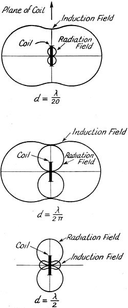
Fundamental Principles and Practice of λ/2π

By Clinton B. De Soto, W1CBD

"The induction field is the field that stays at home." - Prof. R. R. Ramsey

Every time you threw the transmitting switch in pre-war days and sent power surging up into your antenna, two quite distinct electromagnetic fields were set up around it. One of these was the radiation field, the energy in which left the conductor and travelled off into space. The other was the induction field; its energy did not go off into space, but instead returned each time to the parent conductor.

Simply because its energy does travel off into space (and perchance into the intent eavesdropping ears of erstwhile J's, D's, etc.), the radiation field is no longer available for your use. But the once-forgotten induction field, which sends its energy only a little way and then yanks it back again like a yo-yo ball, now offers an interesting field (resemblance to pun purely coincidental!) for experimentation.

Older Than Radio

Even before Maxwell's theory of radiation had been reduced to practice, experimental communi-cation was carried on by means of electrostatic and electromagnetic induction. As early as 1865, Dr. Mahlon Loomis signaled between two mountain tops eighteen miles apart by its use. In the latter 19th century many of the world's greatest scientific minds experimented with inductive effects over distances of a mile or more - Thomas A. Edison, Alexander Graham Bell, Oliver Lodge, A. W. Heaviside and many others.

But with Hertz' demonstration of radiation as a practical phenomenon, the remote induction field came to have little more practical importance in communications than as a source of annoyance to telephone and telegraph men running into cross-talk from parallel wire lines.

Until 1938, that is. In that year Philco engineers, seeking a remote-control tuning system without the inconvenient multi-wire cables and accompanying complexities, evolved the idea of using an inductively coupled r.f. transformer with its primary and secondary spaced as much as 75 feet. The primary of this transformer was supplied from a small battery-powered oscillator, and the voltage induced in the secondary fed a supplementary amplifier in the b.c. set.

Naturally, because of its resemblance to a conventional transmitter and receiver, questions arose concerning the legality of the device. After considerable debate pro and con and a hearing or two, the FCC finally handed down rules cov-ering the subject. For the record, those rules are reproduced here in their entirety:

PROVISIONS GOVERNING THE OPERATION OF LOW POWER RADIO FREQUENCY DEVICES

2.101. General. Pending the acquiring of more complete information regarding the character and effects of the radiation involved, the following provisions shall govern the operation of the low power radio frequency electrical devices hereinafter described.

2.102. Apparatus excepted from requirements of other rules. With respect to any apparatus which generates a radio fre-quency electromagnetic field functionally utilizing a small part of such field in the operation of associated apparatus not physically connected thereto and a distance not greater than , the existing rules and regulations of the Commission shall not be applicable provided:

(a) That such apparatus shall be operated with the minimum power possible to accomplish the desired purpose.

(b) That the best engineering principles shall be utilized in the generation of radio frequency currents so as to guard against interference to established radio services, particu-larly on the fundamental and harmonic frequencies.

(c) That in any event the total electromagnetic field produced at any point at a distance of from the apparatus shall not exceed 15 microvolts per meter.

(d) That the apparatus shall conform to such engineering standards as may from time to time be promulgated by the Commission.

2.103. Exceptions; interference to radio reception. The provisions of sections 2.101 and 2.102 shall not be construed to apply to any apparatus which causes interference to radio reception.

2.104. Inspection and test; certificates. Upon: request, the Commission will inspect and test any apparatus described in sections 2.101 and 2.102, and on the basis of such inspection and test, formulate and publish findings as to whether such apparatus does or does not comply with the above conditions, and issue a certificate specifying conditions of operation to the party making such request.

And so we have the regulatory justification for all such miscellaneous gadgets as the "Mystery Control," wireless phonograph record players, phantom volume controls in p.a, systems and the like. We have also an interesting field for interim experimentation in connection with limited-range communication and remote control devices.

The purpose of this article is not so much to suggest the possibilities, however, as to underline the fundamental principles and to provide a compilation of circuit and design data.

How Radiation and Induction Fields Are Created

It may help in understanding the distinction between the two kinds of fields to review the phenomenon of radiation, as far as that can be reduced to simple, non-mathematical concepts. First of all, consider a simple coil with d.c. flowing through it. A magnetic field is set up around the coil, extending into space for a certain distance with a strength depending on the magnitude of the current. This field has a certain polarity, depending on the direction of current flow.

Now suppose the current is instantaneously cut off. The field collapses and the energy in it returns to the coil. But if, the very instant the current stops flowing in one direction, it starts flowing again in the opposite direction with equal magnitude, an equal and opposite electric field will be set up before the original field can return to the coil. Unable to return home because the new field has forced it out, the original field sets forth on a journey through space.

That constitutes radiation - the successive detachment of one electrical field after another in a series of waves as each is succeeded by another with each reversal of current. In an ideal system with instantaneous reversals, all of the energy in each field would be radiated, and none would return to the coil. In actuality, each succeeding cycle from the a.c. generator feeding the coil represents a slow rise and fall of potential. This gradual building up to peak amplitude and corresponding gradual decay allows time for some of the energy to return to the coil before the new field becomes strong enough to send it away. The slower the rise and fall - i.e., the lower the frequency - the more of the initial energy returns to the coil. Thus at audio or very low r.f, most of the energy succeeds in returning and very little is radiated. At the higher radio frequencies, on the other hand, the cycles come along so fast that the electric field - even though it travels 186,000 miles per second - has little time in which to go out and return, and as a result most of it gets detached and is radiated into space.

The part of the field that returns to the coil is the induction field, while the part that is detached is called the radiation field.

The most obvious difference between the radiation and the induction fields is that the radiation field is the weaker near the antenna and the stronger at a distance. This is illustrated in Fig. 1, based on studies made by Professor Ramsey, which shows the relative strength of the two fields at various relative distances identified in terms of the operating wavelength. Specifically, the radiation field varies inversely as the distance, while the induction field from a coil varies inversely as the cube of the distance. The two fields are always equal at a distance equal to the velocity of light divided by the angular velocity.

This expression will be recognized as that used in the FCC rule to state the maximum distance at which the measured field may not exceed 15 p.v. per meter, to ensure that no interference is caused radio services. Actually, since the two fields are in time quadrature this measured value represents 1.414 times the true value of either field alone, but as far as the receiving antenna or coil is concerned it has no social prejudices and responds to both fields as one.

Thus we have our first design rule - the measured field strength at the distance

                      (1)

must not exceed 15 μV per meter. This distance, expressed in feet, is shown in Fig. 2 for frequencies throughout the region normally used for the purpose.

Calculating Field Strength

The question then arises - how to determine that the field strength at the maximum distance does not exceed the legal limit of 15 μ V per meter? Few amateurs have access to standard signal generators and the rest of the equipment that would be necessary to do the job properly.

However, it is possible to compute the induction field using nothing more than an antenna ammeter of the thermocouple or hot-wire variety and a little care. Knowing the current in and the physical characteristics of the transmitting coil, the field strength at any distance can be worked out by the following formula:

                      (2)

where

E = field strength at the receiving coil in microvolts per meter;

N = number of turns in transmitting coil;

T = radius of transmitting coil in centimeters;

I = current through the transmitting loop in milliamperes; and

d = distance between centers of the transmitting and receiving loops in meters.

This can be stated to give the current required in a given loop to produce the maximum permissible field at any wavelength:

                      (3)

where λ equals the operating wavelength and the other values are the same as in (2).

The physical dimensions of the transmitting coil or primary are not of particular importance if rated current is obtained. The important thing is that both dimensional and electrical measurements be accurately made, and that enough power be available from the oscillator to cause rated current (or slightly less, for a margin of safety) to flow in the coil.

If the current is held at the calculated value, the induction field remains constant regardless of frequency. Unlike the radiation from a coil or antenna, which varies with frequency, the induction field is independent of frequency. In fact, the strength of the induction field is a function solely of the current, the area of the coil, the number of turns and the distance.

The Transmitter

Almost any simple oscillator circuit can be used in the transmitter. Ordinarily not more than 2 or 3 watts input will be required, unless a loop of very few turns and small area is used. One suitable transmitter design was described on page 42 of March, 1942, QST.

Fig.  3 shows an even simpler circuit, suitable for use on c.w. or for sending remote-control pulses. It can also be modulated to perhaps 50% (another 6J5 as modulator would do the job) for voice work. The coupling tap is adjusted to give the calculated current as determined from (2). If more power is required, a 6V6 with No.2 grid tied to plate may be substituted for the 6J5.

The circuit of the Philco "Mystery Control" battery-operated portable control unit is shown in Fig. 4. Used between 350-400 kc., the type 30 tube with 45-volts on the plate gives 130 milli-amperes of r.f. current in the 675-mh. coil (122 mw. power, Q of 216).

The oscillator power transformer should pref-erably have an electrostatic shield between pri-mary and secondary. Transformerless supplies are not advisable for this application because of the excellent possibility of increased radiation. R.f. line filters in the 115-volt leads will help to limit radiation.

In this connection, it is interesting to note that the power wiring, etc., is much more likely to create interference to other radio services by radiation than the emanations from the transmitting loop alone. The efficiency of the coil as a radiator is very poor compared with almost any straight-wire antenna, such as a power line. This is particularly true when the receiver being interfered with is equipped with an antenna rather than a loop.

The Receiving Coil

So much for the transmitter. Let's talk about the receiving coil or the secondary of the induc-tive transformer now. Assuming the loop is located in a known field, the following rules apply:

The voltage induced in the coil is directly pro-portional to the area of the loop (frequency and number of turns remaining constant).

It is directly proportional to frequency (turns and area constant).

It is directly proportional to the number of turns (frequency and area constant).

From the above, it can readily be shown that the induced voltage is proportional to the induct-ance of the coil.

Disregarding strays, the inductance increases as the square of the turns ratio, the area remaining constant. Conversely, the inductance increases as the square of the radius, the number of turns being constant.

All this leads to the conclusion that with a given inductance the induced voltage will be greater the larger the area of the coil. In practice other considerations enter, but the rule holds in general. For maximum sensitivity, therefore, every effort should be made to make the area of the coil as great as possible, and to keep the inductance as high as possible and the capacity - both tuning and distributed - low.

Since the induction-field system is, after all, nothing more than an air-core r.f. transformer - even though the primary and secondary may be spaced thousands of feet - it is quite possible to compute the field induced in the secondary coil at any distance provided only the dimensions of the coils and the current in the primary are known:

                      (4)

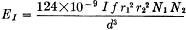
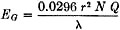
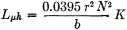
where E_I is the voltage induced in the receiving loop, I the current in the transmitting coil in milliamperes, f the operating frequency in kc., r1 and r2 the radii in centimeters of the transmitting and receiving loops respectively, N1 and N2 the number of turns in the respective loops, and d the distance in meters between them.

The effective signal at the grid of the first amplifier tube when the receiving loop is at the distance λ/2π (coils co-planar) in a 15 μV field can be computed roughly by the following simple relationship:

                      (5)

where E_G is the grid input voltage, r the radius of the receiving loop and N the number of turns. Q refers to the tuned circuit, and can be considered as that of the receiving loop.

The Q of the coil must be made as high as possible, since the voltage applied to the grid of the first amplifier tube in the receiver will be equal to the induced voltage times the Q of the tuned circuit. This is determined by a number of factors, including wire size, shape and insulation. At the frequencies normally used Litz wire would be desirable, but unfortunately it is not now readily available. Any available solid wire between No. 24 and 30 will result in a satisfactory coil. Smaller wire than No. 32 or larger than No. 20 is not recommended for these frequencies.

The large diameter required in coils of this type makes it impossible to use the form factor normally considered best at the frequencies in use. However, by using single-layer windings, spacing the wire slightly or using double-cotton-covered wire, and keeping the insulating or supporting material in the coil to a minimum, a coil of good Q can be made.

Calculating Inductance of Loops

The inductance of large-diameter coils is difficult to calculate exactly, but it can be worked out with fair accuracy by using Nagaoka's formula:

                      (6)

where r is the radius in cm., N the number of turns, b the winding length of the coil in cm. and K a constant obtained from Fig. 5.

This formula is accurate only for single-layer solenoid coils, but approximations sufficiently close for ordinary work (there'll be some trimming and paring anyway) can be made by taking the periphery of coils of other shapes and dividing by 2π to obtain T. Thus a square loop 30 inches on a side, an equilateral triangle with 40-in. legs or a circle with a circumference of 120 inches all have the same value of r = 19.1 inches.

In the case of spiral coils (as in Fig. 6), for r use the mean radius - i.e., one-half of the inside diameter plus b.

Fig.  6 shows two satisfactory methods of loop construction. For the higher frequencies large cardboard containers, such as oatmeal boxes, make suitable forms. Self-supporting basket-weave coils can be made with heavy wire by arranging wooden pegs in a circle and interwinding a solenoid coil around them in similar fashion to the "spider-web" spiral winding of Fig. 6 - (A).

The Receiver

Undoubtedly the toughest problem in setting up an induction-field system is the receiver, at least if you aren't going to be satisfied with anything less than a completely independent unit. It takes a good bit of gain to build 15 microvolts (more or less) into a usable signal, and gain means stages and tubes - and sometimes trouble. It's a good idea, too, to keep the selectivity of the amplifier high, because reduced bandwidth means reduced noise, and the ultimate limit in the useful range is determined by the equivalent sideband noise input ratio.

The best system without doubt is the use of a low-frequency converter and your present communications receiver. The unit described by Goodman in the March issue, beginning on page 15, can be applied to the present problem. The tuned circuits must, of course, be modified to fit the chosen operating frequency, but that isn't much of a job, particularly since most induction-field work will be more or less fixed-tune, anyway, and there won't be any tracking problem. And stage might be desirable to improve the signal-to-noise ratio if work is to be done at the extreme limit of the useful range, but all in all the complication hardly seems worthwhile.

If a receiver is built especially for the job it logically becomes a straightforward r.f. amplifier, with two or three stages depending on the frequency and required sensitivity, each stage individually tuned. In designing such a receiver three quantities should be known - input signal voltage, E1, gain per stage, and required voltage out of the detector, Eo. Divide Eo by E1 to get the overall gain required, and then in turn divide that figure by the stage gain to arrive at the number of stages needed.

I.f. transformers constitute logical interstage coupling devices. Standard replacement transformers are available for frequencies such as 125, 175, 262, 375, 455 kc., etc.: consult a serviceman's manual for types and sources.

Those who have ancient b.c.l. superheterodynes or parts therefrom kicking around, or who have access to such sets in local radio graveyards, may find themselves all set up with a gold mine.

The old low-frequency i.f. transformers - standard i.f.'s in the '20's ranged from 30 to 115 kc. - should work well in this job.

Fig. 7 shows the circuit of a receiver built around a set of small 175-kc. u.f. transformers and used in the 150-200-kc. band. It was made originally for remote-control purposes, and therefore ends in a carrier-operated relay tube. When a signal is received the diode biases the grid of the 6R7 triode, reducing the plate current and releasing the relay contacts. For communication work the triode could be connected as an ordinary audio amplifier, by the addition of a 0.01-μfd. coupling condenser and 1-megohm grid resistor. A transformerless power supply is used.

Even at 150 kc, the useful range is only a fraction of a mile, and therefore it is the lower frequencies that look most attractive for induction-field work. If no transformers suitable for those frequencies are available, tuned impedance coupling can be used as shown in Fig. 8. Ordinary lattice-wound r.f. chokes may be used as coils.

With this type of circuit the gain per stage is approximately:

                      (6)

where Gm is the amplifier tube transconductance in mhos, I is the operating frequency in kc., L the inductance in millihenries and Q that of the coil (50-100 for ordinary r.f. chokes, 100-200 for honeycomb coils and solenoids, 150-300 for good powdered-iron core coils).

For maximum gain the operating frequency should be chosen so that the coil tunes to resonance with minimum tuning capacity. Thorough shielding and bypassing of each stage is recommended as high-gain multi-stage amplifiers of this type are more than a little inclined to instability unless carefully handled

Posted December 14, 2020
(updated from original post on 9/13/2012)