Low-Noise Receiver Performance Measurements, March 1969 Electronics World

I was first introduced to the concept of receiver noise figure at the start of my engineering career in 1989 at General Electric Aerospace Electronics Systems Division (AESD) in Utica, New York. During my four years in the U.S. Air Force (1978 to 1983) working on airport surveillance and precision approach radars, I do not recall having ever heard the term noise figure or noise temperature. We did signal to noise and signal sensitivity measurements as part of the normal maintenance, but the terms never arose. Ditto for my courses at the University of Vermont. We never did cascade parameter calculations for noise figure, intercept points, compression points, etc. That is primarily the realm of practicing design engineers, evidently. Maybe I was asleep in class at tech school (Keesler AFB, Mississippi) and UVM the day(s) it came up.

I would be remiss without taking the occasion of this article to promote my Wireless System Designer software that provides an incredible level of RF system design calculations for a mere $45. That price doesn't even amount to a single hour of your company's billing time for your work.

Noise-figure measurements are easy to make; it's an efficient, simple, and accurate method of determining receiver performance.

During the past decade, low-noise receivers have become practical devices and are widely used in commercial and military communications systems.

Fig. 1 - Thermally agitated electrons cause noise in receiver input circuits. Johnson noise reduces signal intelligibility.

However, the literature which describes their performance continues to confuse many engineers and technicians. In this article, two of the most meaningful receiver sensitivity terms-"noise figure" and "effective noise temperature" (ENT) - have been related and the problems involved in gauging the actual sensitivity of a receiver rated with a "negative" noise figure shown. The hot/cold body standard technique, a testing procedure specifically designed to measure the noise figure or ENT of low-noise receivers, is also discussed.

Both noise figure and ENT are currently used by engineers to indicate the performance of low-noise radio-frequency amplifiers. Most engineers prefer to use ENT for the extremely low noise devices and noise figure for conventional receivers (for example, those with noise figures greater than 6 decibels).

The noise figure of a receiver represents a comparison between an actual receiver and its theoretically perfect counterpart. The term "noise figure" was first used in 1940 by radar engineers making receiver sensitivity measurements. They found that a receiver's bandwidth had a disturbing effect on sensitivity readings: the narrower the bandwidth, the better the reading. But when sensitivity was measured using gas or thermal noise generators, the bandwidth did not affect the readings; low receiver gain showed up as an abnormal noise figure.

The noise figure of a network is defined by the IEEE as the ratio of the total noise power available at the output port when the input termination is at 290° Kelvin to that portion of the total available noise power produced by the input termination and delivered to the output by the primary signal channel. It will become apparent from the discussion clarifying this definition that noise figures below zero decibels are automatically excluded. Therefore, the "perfect" amplifier has a noise figure of 0 dB.

Fig. 1 illustrates the case of the perfect receiver with its input network at a temperature of 290° K (63° F). The resistance (R), which represents the impedance of the feed, generates a noise voltage called Johnson noise. This noise results from the random motion of thermally agitated free electrons. Although this noise voltage has an infinitely wide bandwidth, we are only interested in the signals which fall within the receiver's bandwidth because only these noise voltage signals pass through the amplifier and register on the power meter. It is only this noise with which the incoming signals have to compete.

When a perfect receiver is matched to an input network, the input noise power (in watts) can be expressed as:

where k is Boltzmann's constant (1.38 X 10^-23 joule/degree Kelvin), B is noise bandwidth of the amplifier in Hz, and T is 290° K.

The noise bandwidth of the network is not the same as the half-power bandwidth normally given in performance specifications; rather, it is somewhat wider and normalized at the network's center frequency. In some cases, it is quite close to the 3-dB bandwidth, but sometimes it is as much as 1.57 times the half-power figure. However, as long the receiver is tested with very wide thermal or gas noise sources, this difference is of no great concern.

Fig. 2 - This graph can be used to convert effective noise temperature measurements to their true noise figure value.

A power meter hooked to the output of a perfect receiver as shown in Fig. 1 would read a power N₁ equal to kBTG, where G is the power gain of the receiver. However, a receiver contributes noise of its own (ΔN) so that an actual receiver's output (N₂) is kBTG + ΔN. Specifically, the term noise figure (F) is a ratio that compares a receiver with its ideal counterpart and is equal to the noise power output from an actual receiver with its input network at 290° K, divided by the noise power output from an ideal receiver with its input network at 290° K. Or,

If the device under test were perfect, ΔN would be zero and the receiver's noise figure would reach the limit of unity or 0 dB.

The effective noise temperature is more difficult to determine. When a receiver's input-network temperature is raised above 290° K, the random noise generated by the network increases and the output noise power rises to a new value of N₂. The ENT is the number of degrees that the input network's temperature had to be raised before the receiver's output reached the new value of N₂.

When the expression for N₂ in equation (2) is resolved into thermal components, the equation has the following form:

Component T is the noise from the receiver's input network (at 290° K) and T_e is the internally generated amplifier noise or ENT:

If the receiver contributed no noise of its own, T_e would be zero and F would again be unity or 0 dB. When the kBG terms of equation (4) are cancelled, we are left with a simple expression for noise figure in terms of ENT:

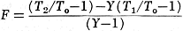
Fig. 3 - Measurement errors are greater at the lower noise figure values. This graph is used when the input network behaves as though it were operating at other than 290° Kelvin. In the example, a 5-dB measurement is corrected to read 6 db.

ENT is an absolute quantity in degrees Kelvin defined by the relationship T_e = (F - 1)T. It is emphasized at this point that ENT is not the physical temperature of the receiver's input network; it is an apparent temperature that is representative of an amplifier's internally generated noise. Fig. 2 is a graph for converting ENT ratings to noise figure and vice versa.

We have excluded negative values from our definition of noise figure and have, until now, assumed that all networks behave as though they were at 290° K. Quite frequently, however, a network acts as though it were at a lower temperature. The result is an abnormal noise figure which, by conventional measuring techniques, is difficult to distinguish from an acceptable noise figure measurement. If, for example, the input circuit behaved as though it were at a temperature lower than 290° K and the amplifier itself contributed little noise, the quantity of noise proportional to kBTG + ΔN, which conventional techniques measure, is small. On the other hand, the quantity kBTG, which conventional techniques calculate, will be considerably greater than its true value, If the amplifier's true noise figure is low enough and the network's temperature deviation from the assumed 290° K is large enough, the calculated value almost equals the measured values.

The magnitude of the measurement error depends upon the true noise figure. Measurement errors increase rapidly as lower noise figure values are reached. Fig. 3 is a graph of the equation used to correct the values of noise figures. In the example shown on the graph, the 5-dB noise figure measurement was made while the input network behaved as though it were operating at 100° K. The correction is +1 dB so that the true noise figure, referenced to 290° K, is 6 dB.

Hot/cold body standards enable the previously described measurement difficulties to be overcome. While not suitable for the amateur or small shop owner, they enable the manufacturer to test his products and assign them a proper noise figure or ENT.

Hot/cold body standards use two resistive elements, one immersed in liquid nitrogen at 77.3° K and the other in a temperature-controlled oven at 373.1° K. The noise power (in watts) from either resistor equals kBT, where T is the temperature of the particular resistor in degrees Kelvin and k and B are the quantities described in equation (1) . The testing procedure is illustrated in Fig. 4.

where To is 290° K, T₁, is 77.3° K, T₂ is 373.1° K, and Y is N₂/N₁. By measuring N₁ when the receiver's input network is at a known temperature (T₁) and measuring N₂ when it is terminated at T₂, the corrected noise figure can be calculated directly by equation (6).

Fig. 4 - Accurate noise figure measurements can be obtained by switching a receiver between an input network immersed in liquid nitrogen and a network in a temperature-controlled oven.

Although hot/cold body standards were specifically developed to clear up the problems that arose when low-noise amplifiers were tested by conventional methods, they have, unfortunately, also been used as a means to further improve noise figure specifications. In examining the literature, one can find examples of noise figures specified as the ratio of ENT to the nitrogen bath temperature. Such ratings are usually presented as negative noise figures. Another practice, even more misleading because it yields a positive noise figure, is that of specifying noise figure as the ratio of the nitrogen bath temperature plus ENT to the bath temperature.

A further difficulty, not necessarily associated with the hot/cold body standards, is the tendency of some experimenters to specify noise figures based on reference temperatures other than 290° K.

Noise figure and ENT are equivalent ways of describing low-noise receiver performance. For absolute comparisons to be made between devices, however, both terms must be referenced to the standard temperature of 290° K.

Low-Noise Receiver Performance MeasurementsMarch 1969 Electronics World

Low-Noise Receiver Performance Measurements
March 1969 Electronics World