Plotting Coverage Circles For Satellite Communications, January 24, 1964 Electronics Magazine

One of the major advantages of the age of powerful personal computers - be they in the form of desktop systems, tablets, or smartphone apps - is that for most computation-intensive tasks there only needs to be one or maybe at most a few people smart enough to know how to do them. Everyone else who has to perform the task just needs to be able to input the proper parameters to ensure a useful output. That is a significant statement, because in the days before ubiquitous computer availability and incredible computing power, highly capable engineers, scientists, analysts, and mathematicians either had to be on staff or an expert external resource was used for difficult and/or time-intensive tasks. Over time, fewer and fewer people are needed to produce very precise and reliable results. In many ways, other than the creative intuition involved in concept, creation, and execution, a large part of the product design and planning phases have been automated with the help of very capable software. This 1964 Electronics magazine article about plotting of satellite ground coverage maps is a good example.

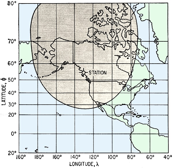
Fig. 1 - Coverage of a ground station located at 55 degrees north latitude.

Graphical method solves most circular-orbit cases to determine possibility of communications.

Continuing announcements of communication satellite plans give point to an article that shows how, with simple computation and available charts the planner, engineer and even the space hobbyist can determine the coverage circle of a ground station for a satellite in a nearly circular orbit

Plotting the coverage circle of a ground station that is in communication with a satellite is a tedious task because of the extreme distortion of many map projections, as illustrated in Fig. 1. A graphical technique has been developed that greatly facilitates this operation. It involves drawing the coverage circle as a semicircle on a work sheet and then transferring coordinate values to the map projection in use.

For this purpose, the surface station is taken to be located at 0 degrees longitude and Φ_s degrees latitude. The radius of its coverage circle subtends the angle a at the center of the earth. The latitude and longitude, Φ and λ, of points on the circumference of this circle satisfy the equation¹

Rather than solve this equation for specific pairs of coordinates, the engineer can use a compass to draw the coverage circle on the work sheet of Fig. 2A or 2B, depending upon the station coordinates. Figure 2A presents a polar stereographic projection of the earth and Fig. 2B shows a meridional stereographic projection of the earth with the pole of the projection centered on the equator. A circle drawn on the earth about a point representing the station appears on the stereographic projection as a circle with its center displaced in latitude from the ground site.

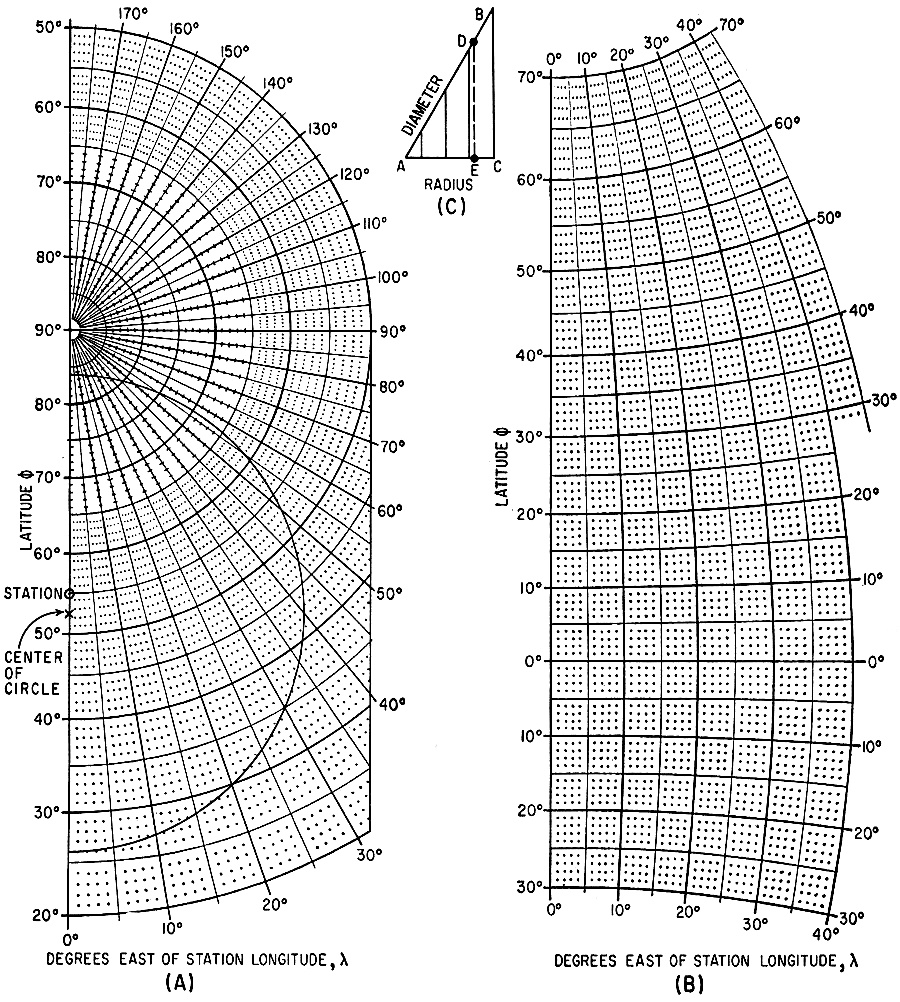
Fig 2. - POLAR stereographic projection (A) stereographic meridional projection (B) and representative radius scale (C).

The central angle of the coverage circle a can be determined from Fig. 3 for a particular elevation angle above the horizon for a satellite in a near-circular orbit at an altitude of H nautical miles. For example, a central angle of 29 deg occurs for 0 deg elevation angle when the orbital altitude is approximately 490 nautical miles.

Example - The circle drawn on Fig. 2A is for a station latitude of 55 deg and circular coverage α = 29 deg. The procedure for drawing this circle is as follows

2. α = 29 deg determines the northern and southern limits of the circle on the zeroth meridian as 55 deg + 29 deg = 84 deg N and 55 deg - 29 deg = 26 deg N.

3. A caliper is set at the diameter length between 84 deg N and 26 deg N on the zeroth meridian of Fig.2A.

4. The caliper diameter AD is marked on scale AB of Fig. 2C and the corresponding circle radius AE is measured on the associated radius scale AC, as illustrated.

5. Measure the radius length AE from either the 84 deg N or the 26 deg N limit on the zeroth meridian of Fig. 2A to locate the center of the circle on the map.

6. The semicircle is drawn on Fig. 2A using the radius AE and the center location of step 5 above.

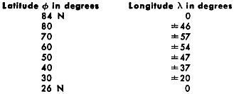
The coordinates of points on the circle read from Fig. 2A are shown in Table I. If the actual longitude of the station is 130 deg W, the table leads to the distorted coverage zone shown in Fig. 1 for a Mercator projection.

When the ground station is nearer the equator, the semicircle may extend beyond the limits of Fig. 2A. For this case, it should be drawn on the meridional stereographic projection of Fig. 2B, using the same sequence of steps outlined above. Both Fig. 2A and 2B are usable for stations in southern latitudes by reading all latitude values as south, rather than north. When the central angle exceeds 30 deg, a different graphical procedure may be employed.² Neither the technique described here, nor that of the footnote reference, applies for the coverage in a highly elliptic orbit, since the limits on the surface of the earth do not lie on a circle about the ground station.

Fig. 3 - Central angle upon which coverage circle depends is determined from graph.

Scaling Radius - Figure 2C provides a convenient means of dividing a length (the measured diameter of the circle) by two to obtain a direct measure of the radius. The figure comprises two lines that intersect at an angle of 60 deg. This can be redrawn enlarged with intermediate ticks to facilitate accuracy.

Alternatively, the latitude of the center of the circle may be computed by means of the relation

Thus, for the example presented, Φ_s = 55 deg, α = 29 deg, and slide rule computation gives Φ_center = 52.5 deg, in agreement with the location on Fig. 2A.

Another simple means of locating the center of the circle is to measure the distance between the northern and southern limits on the zeroth meridian, established in step 2 of the example. Division of this distance by 2 then gives the linear measure of the separation of the center from either of the established limits.

(1) D. Levine, "Radargrammetry", p 300, McGraw-Hill Book Co., New York, N. Y., 1961.

Since the Fig. 2A is a polar stereographic projection, the coverage circles may be drown on any standard map that employs this projection. The following maps are listed in order of decreasing scale factor:

(1) Scale 1:10,500,000, six-sheet wall map of the world, size 108 in. by 126 in., USAF Strategic Outline Charts, No. SO-17.

(2) Scale 1:17,750,000, size 51 in. by 30 in., USAF Strategic Planning Charts, Northern hemisphere - No. SP-2; Southern hemisphere-No. SP-3.

(3) Scale 1:24,000,000, size 38 in. by 36 in., Northern hemisphere USAF Strategic Outline Chart, No. SO-16.

(4) Scale 1:48,000,000, size 19 in. by 18 in., Northern hemisphere, USAF Strategic Outline Chart, No. SO-16a.

(5) Scale 1:63,000,000 at 60 deg. N. lat., Weather Plotting Chart, Northern hemisphere, No. AWS-WPC-6-63-1, (Aeronautical Chart and Information Center).

The meridional stereographic projection, Fig. 2B, also corresponds to a standard projection, so the coverage circle may be drawn on any appropriate map. The choice now is more limited than for the first figure. For this purpose, there is available the National Geographic map of the Atlantic Ocean, scale 1:20,000,000, size 25 in. by 31.25 in. (Sept. 1941).

For this chart, the circle is centered on the 40th meridian, which corresponds to the vertical line on the left side of Fig. 28. Continental outlines and other geographic features are ignored when using this map as a work sheet.

Plotting Coverage Circles for Satellite Communications January 24, 1964 Electronics Magazine

Plotting Coverage Circles for Satellite Communications
January 24, 1964 Electronics Magazine