Custom Search

Over 9,000 pages indexed!

Your Host

Kirt
Blattenberger
... single-handedly
redefining what an
engineering website should be.

Carpe Diem!
(Seize the Day!)

5CCG (5th MOB):
My USAF radar shop

Hobby & Fun

Airplanes and Rockets:
My personal hobby website

Equine Kingdom:
My daughter Sally's horse riding business website - lots of info

Doggy Dynasty:
My son-in-law's dog training business


•−• ••−• −•−• •− ••−• • RF Cafe Morse Code >Hear It<
Job Board
About RF Cafe©
RF Cafe E-Mail

Product & Service Directory		Engineering Jobs
Personally Selected Manufacturers		Employers Only (no recruiters)

Cascaded 1 dB Compression Point (P1dB)

When operating within the linear region of a component, gain through that component is constant for a given frequency. As the input signal is increased in power, a point is reached where the power of the signal at the output is not amplified by the same amount as the smaller signal. At the point where the input signal is amplified by an amount 1 dB less than the small signal gain, the 1 dB Compression Point has been reached. A rapid decrease in gain will be experienced after the 1 dB compression point is reached. If the input power is increased to an extreme value, the component will be destroyed.

P1dB_output = P1dB_input + (Gain - 1) dBm

1 dB Compressor Point (P1dB) - RF Cafe

Passive, nonlinear components such as diodes also exhibit 1 dB compression points. Indeed, it is the nonlinear active transistors that cause the 1 dB compression point to exist in amplifiers. Of course, a power level can be reached in any device that will eventually destroy it.

Graph of relationship between IP2, IP3, and P1dB - RF Cafe

A common rule of thumb for the relationship between the 3rd-order intercept point (IP3) and the 1 dB compression point (P1dB) is 10 to 12 dB. Many software packages allow the user to enter a fixed level for the P1dB to be below the IP3. For instance, if a fixed level of 10 dB below IP3 is used and the IP3 for the device is +30 dBm, then the P1dB would be 18 dBm.

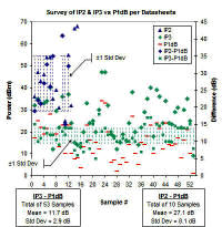
In order to test the theory, IP3 and P1dB values from 53 randomly chosen amplifiers and mixers were entered into an Excel spreadsheet (see table below). The parts represent a cross-section of silicon and GaAs, FETs, BJTs, and diodes, connectorized and surface mount devices. A mean average and standard deviation was calculated for the sample.

As it turns out, the mean is 11.7 dB with a standard deviation of 2.9 dB, so about 68% of the sample has P1dB values that fall between 8.8 dB and 14.6 dB below the IP3 values. What that means is that the long-lived rule of thumb is a pretty good one. A more useful exercise might be to separate the samples into silicon and GaAs to obtain unique (or maybe not) means and standard deviations for each.

An interesting sidebar is that where available, the IP2 values were also noted. As can be seen in the chart, the relationship between IP2 and P1dB is not nearly as consistent.

Of equal motivation for the investigation was the desire to confirm or discredit the use of the noise figure and IP3 type of cascade formula for use in cascading component P1dB values. As discussed elsewhere, the equation for tracking a component from its linear operating region into its nonlinear region is highly dependent on the entire circuit structure, and one model is not sufficient to cover all instances. Indeed, the more sophisticated (pronounced “very expensive”) system simulators provide the ability to describe a polynomial equation that fits the curve of the measured device. Carrying the calculation through many stages is calculation intensive. Some simulators exploit the rule of thumb of IP3 versus P1dB tracking and simply apply the IP3 cascade equation to P1dB. As with other shortcuts, as long as the user is aware of the approximation and can live with it, it’s a beautiful thing.

Cascading P1dB Values in a Chain of Components

Calculating the cascaded values for P1dB for the system budget requires the following operation based upon ratios for gain and P1dB (do not use decibel values). The standard format for indicating decibel values is to use upper case letters, i.e., OP1dB for units of dBm. The standard format for indicating watt values is to use lower case letters, i.e., op1dB for units of mW or W.

Cascaded components for calculating IP2 and IP3 - RF Cafe

A Typical Chain of Cascaded Components

This equation gives the method for calculating cascaded output p1dB (op1dB) values based on the oip3 and gain of each stage. When using the formula in a software program or in a spreadsheet, it is more convenience and efficient to calculate each successive cascaded stage with the one preceding it using the following format:

Cascaded op1dB equation formula - RF Cafe

These formulas are used to convert back and forth between input and out P1dB values:

P1dB_output = P1dB_input + (Gain - 1) dBm
P1dB_input = P1dB_output - (Gain - 1) dBm

Table of IP3, IP2, and P1db Values from Vendor Datasheets
Type	Mfg	Model	IP2	IP3	P1dB	P1dB-IP2	P1dB-IP3
Amp	Amplifonix	2001	36	32	17	19	15
Amp	Amplifonix	8701	47	35	25	22	10
Amp	Amplifonix	5404	43	33	22	21	11
Amp	Couger/Teledyne	A2C5119	46	33	19	27	14
Amp	Couger/Teledyne	A2C4110	54	34	21.5	32.5	12.5
Amp	Couger/Teledyne	A2CP14225	54	40	28	26	12
Mixer	Couger/Teledyne	MC1502	35	12		35	12
Amp	Mimix Broadband	CMM-4000	39	29.5	19		10.5
Amp	Mimix Broadband	CMM-1110	31	22	13		9
Amp	M/A-COM	A101	64	36	23	41	13
Amp	M/A-COM	A231	25	22	10	15	12
Amp	M/A-COM	AM05-0005	55	37	23	32	14
Amp	M/A-COM	SMA411	32	24	10		14
Mixer	Polyphase	IRM0714B	67	15	7.6		7.4
Mixer	Polyphase	IRM1925B	68	14	8		6
Mixer	Amplifonix	M53T		13	3.5		9.5
Amp	JCA	JCA01-301		20	13		7
Amp	JCA	JCS02-332		33	23		10
Amp	Mimix Broadband	XL1005		24	16		8
Amp	Technology Distribution	0600-0007		25	10		15
Amp	Technology Distribution	0600-0025		20	15		5
Amp	Technology Distribution	0600-0024A		30	12		18
Amp	Stealth Microwave	SM3436-34HS		47	34		13
Amp	Stealth Microwave	SM1925-33		47	33		14
Amp	M/A-COM	MAALSS0045		32	20		12
Mixer	M/A-COM	CSM1-10		19	6		13
Mixer	M/A-COM	M5T		18	7		11
Mixer	Marki Microwave	M1-0204L		12	2		10
Mixer	Marki Microwave	M1R-0726M		15	5		10
Mixer	Polyphase	SSB2425A		19	8		11
Amp	Triquint	TGA2512-SM		16	6		10
Mixer	Triquint	CMY 210		24	14		10
Amp	Miteq	AFS3-00500200-27P-CT-6		38	27		11
Amp	Milliwave	TMT4-060-180-35-10P-2		20	10		10
Amp	Milliwave	TMT6-500-750-100-5P-5		14	5		9
Amp	Milliwave	AMT4-060-180-40-10P-1		22	15		7
Amp	Skyworks	SKY65013-70LF		29	14		15
Amp	Skyworks	SKY65015-92LF		35	18		17
Mixer	Synergy	FSM-2		40	23		17
Mixer	Synergy	SGM-2-17		18	10		8
Amp	Microwave Technology	MwT-A989		39	24		15
Amp	Hittite	HMC376LP3		36	21.5		14.5
Amp	Hittite	HMC564		24	12		12
Mixer	Hittite	HMC399MS8		34	24		10
Amp	RFIC	RFISLNA01		24	14		10
Amp	RFMD	NBB-302		23.5	13.7		9.8
Amp	RFMD	RF2878		29	14.4		14.6
Amp	NuWaves	NILNA-GPS		31	17		14
Amp	MCL	AMP-15		22	8		14
Amp	MCL	ZFL-500HLN		30	16		14
Amp	MCL	ZQL-900LNW		35	21		14
Mixer	MCL	MCA-19FLH		25	10		15
Mixer	MCL	MCA-1-12GL		9	1		8
					Mean	27.05	11.6566
					StdDev	8.1	2.9
					Samples	10	53

Cascading of 1 dB Compression points is not a straightforward process, since the curve followed from linear operation into saturation is dependent upon the circuit characteristics. RF Workbench uses an approximation to model the transition from linear operation through saturation.

Click here to view an
example cascaded system.

RF Cafe Software

RF Cascade Workbook

RF system analysis including
frequency conversion & filters

Smith Chart™ for Excel
Smith Chart™ for Visio
RF & EE Symbols Word
RF Stencils for Visio

A Disruptive Web Presence™

Custom Search

Over 9,000 pages indexed!

Read About RF Cafe
Webmaster: Kirt Blattenberger
KB3UON

Product & Service Directory
Personally Selected Manufacturers

RF Cafe T-Shirts & Mugs
Calculator Workbook
RF Workbench

Please Support My Advertisers