|
|||||||||||||
 |
|||||||||||||
Antenna Matching with Line Segments |
|||||||||||||
How RF circuits work have long been referred to as "black magic," even sometimes by people who fully understand the theory behind the craft. To me, the ways in which a transmission line - be it coaxial cable, microstrip, or waveguide - can be manipulated and controlled with various combinations of lengths and terminations is what most qualifies as "magic." Sure, I know the equations and understand (mostly) what's happening with incident and reflected waves, etc., and how the impedance and admittance circles of a Smith chart graphically trace out what's happening, but you have to admit there's something mystical about it all. Fortunately, Mr. John Marshall published this "Antenna Matching with Line Segments" article in the September 1948 issue of QST magazine. Antenna Matching with Line Segments Design Formulas for Wide-Range Matching By John G. Marshall, W0ARL
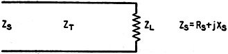
Fig. 1 - Simple transmission line segment. Although design charts for determining the length and position of a matching stub have been available for some time, their use is restricted to the special case where the line and stub have the same characteristic impedance. This article treats the linear matching transformer from a more general standpoint, giving considerably more latitude in the choice of matching arrangements. Many methods of matching the antenna to the transmission line have been described, but with the exception of the Q-section transformer, very little design information has been published on those that employ a section of line as a transformer. Practically nothing has been published on the actual design of the series-balanced network. The same holds true for the shunt-balanced network, except for what has been written about the simplest form of the matching-stub system. This article was prepared for the purpose of making available simple formulas for designing all types of networks that employ a section of line as a transformer, whether series- or shunt-balanced, including those in which the transformer section and/or the stub, if used, have values of characteristic impedance different from that of the transmission line. Early design of the matching-stub network consisted of connecting a λ/4 section of line to the antenna and attaching the transmission line at the point that minimized the standing waves. In many cases, depending upon the ratio of antenna driving-point impedance to transmission-line characteristic impedance, this procedure did not sufficiently reduce the standing-wave ratio. More recently, graphical solutions, which require the transmission line, transformer section and the stub itself to have the same value of characteristic impedance, have appeared.1 As will be seen, the formulas included here are not restricted in the above manner; and, if desired, each element of the network may have a different value of characteristic impedance.
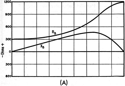
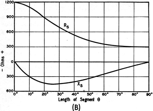
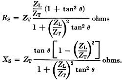
Fig. 2 - Values of input resistance, RS, and input reactance, XS, at various segment lengths. At (A) is shown a typical case where ZL < ZT (ZL = 300, ZT = 600), and in (B) ZL > ZT (ZL = 1200, ZT = 600).
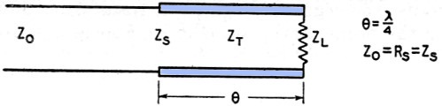
Fig. 3 - Q-section transmission line transformer. Since these networks employ the transformer action of a segment of line terminated by an impedance not equal to the characteristic impedance, a brief review of line segments having lengths up to λ/4 is in order.1 Line segments possess many interesting and valuable properties and those important to these networks are to follow. When a section of line like that in Fig. 1 is terminated by a purely resistive impedance, ZL, not equal to the characteristic impedance, ZT, the sending-end impedance, ZS, contains a reactance component, XS, as well as a resistance component, RS, at all lengths, θ, except exact multiples of λ/4. ZS is actually the effective value of ZL as seen through the section of line. Input Reactance of Segment Except when ZL = ZT, gradually increasing θ from zero causes the reactance, XS, that appears at the sending end to rise gradually from zero to a maximum and then fall back to zero as θ reaches λ/4. XS is zero when θ is zero or λ/4, and is maximum when θ is one certain intermediate value. This maximum becomes smaller as ZL and ZT approach equality, to the point where XS is zero at any value of θ when ZL becomes equal to ZT. The actual value of this maximum, or the value of θ that causes it, is unimportant here. At lengths less than λ/4, XS is inductive when ZL < ZT; and when ZL > ZT, XS is capacitive. Input Resistance of Segment When ZL < ZT, gradually increasing θ from zero causes the resistance, RS, appearing at the sending end to rise gradually from a minimum to a maximum, as θ reaches λ/4. The minimum value, which is equal to ZL, occurs when θ is zero, while the maximum value, which is equal to ZT2/ZL, occurs when θ is &lambda/4. The greater the ratio ZT/ZL and the nearer θ is to λ/4, the greater is the step-up transformer ratio. When ZL> ZT, gradually increasing θ from zero causes RS to drop gradually from a maximum to a minimum, as θ reaches λ/4. This maximum, which is equal to ZL, occurs when θ is zero, while the minimum, which is equal to ZT2/ZL, occurs when θ is λ/4. The greater the ratio ZL/ZT and the nearer θ is to λ/4, the greater is the step-down transformer ratio. A graphical representation of these effects is given in Fig. 2. Fig. 2-A shows how the resistance and reactance vary along a piece of 600-ohm line terminated in 300 ohms, and Fig. 2-B shows the variation along a 600-ohm line with a 1200-ohm termination. The shapes of the curves would be the same for any similar ratios of ZL and ZT - only the "Ohms" scale would change. Irrespective of whether the transformer ratio is step-up or step-down, as ZL and ZT approach equality the smaller this ratio becomes. This may be carried to the point where ZL, ZT, maximum RS and minimum RS all are equal. When this happens there are no standing waves, no XS, and consequently, a transformer ratio of 1 to 1 at any value of θ. From the above, it is seen that a variety of transformer ratios is available by selecting various combinations of θ and ZT.
Since RS, not XS, handles the power, the trans-former ratio between ZL and RS is the heart of all antenna-matching systems that employ the transformer action of a section of line. But in order to use this transformer action θ must be fixed at some odd multiple of λ/4, unless some other means is provided to balance out XS. Three general methods of treating the above reactive condition are illustrated in Figs. 3, 4 and 5. Q-Section Transformer Fig. 3 shows the popular Q-match, which is covered in all the handbooks. It is briefly described here merely to show its behavior and relationship to the other networks employing the linear transformer. In this system, a λ/4 segment is selected having a value of ZT that produces a ZS containing an RS equal to the characteristic impedance, Z0, of the transmission line. Since θ is an exact multiple of λ/4, ZS is purely resistive and there is no XS to balance out. With given values of ZL and Z0,
Since ZT is the only variable and there are limits to the useful range of characteristic impedances, the Q-match can be used to accommodate only part of the many combinations of ZL and Z0 encountered.2 As will be seen, the other networks employing the linear transformer are not limited in this respect. Series-Balanced Network In the series-balanced network of Fig. 4, a segment is selected which has a convenient value of ZT (usually equal to Z0) and of such length, θ, that ZS contains an RS equal to Z0 In other words, the segment becomes a transformer having the proper ratio to make ZL appear equal to Z0 This condition is fully accomplished by balancing out the reactance component, XS. by a series reactance, XBS, of equal ohmic value but of opposite sign. Then the line looks into an impedance equal to its own Z0. With a suitable type of line selected for the transformer section.2 the correct length, θ, and the total XBS necessary to bring about the above conditions, may be found from3:
When the same material is selected for the transformer section as for the transmission line - which is most common and usually permissible - ZT will equal Z0, and simpler formulas may be used.2 In these cases, formulas (1) and (2) reduce considerably, and values of θ and total XBS may be found from:
XBS = tan θ (ZL - Z0) ohms. (4)
Fig. 4 - Series-balanced network. In the series-balanced network, the total XBS should be equally divided between the two legs of the circuit. It is important to note that when a capacitive balancing reactance is used each individual reactor must contain twice the total capacity in order to contain half the total reactance. The unmodulated peak voltage across each individual balancing reactor is
Shunt-Balanced Network In the shunt-balanced network of Fig. 5, a segment is selected which has values of ZT and θ that render a ZS whose equivalent parallel impedance, ZP, contains a parallel resistance component, RP, equal to Z0. The parallel re-actance component, XP, is balanced out by a parallel reactance, XBP, of equal ohmic value but of opposite sign. Then the line looks into a pure resistance equal to its own Z0. With a suitable type of line selected for the transformer section,2,3 the correct values of segment length, θ, and parallel balancing reactance XBP, necessary to bring about the above conditions may be found from
As in the series-balanced network, if the same material is selected for the transformer section as for the transmission line, ZT will equal Z0 and simpler formulas may be used.2 In these cases, formulas (5) and (6) reduce considerably, and values of θ and XBP my be found from
The unmodulated peak voltage across XBP is
Table I - Proper Formulas for Finding Length of Transformer Section and Value of Balancing Reactance * When a stub is desired at XBP, β is found from (9) or (10). Linear Shunt Reactors The shunt-balanced network is especially suited to the use of a linear balancing reactor, such as that made of a segment of open or closed line. It is quite convenient that any practical value of characteristic impedance, ZC, may be selected for the linear reactor or stub. After selecting a value for ZC, the necessary length, β, to give the required value of XBP, may be found from
and
for the open and closed stub, respectively. The Handbook1 shows that when β is less than λ/4, an open stub is a capacitive reactance while a closed stub is an inductive reactance. Formulas (9) and (10) bear this out. NOMENCLATURE Z0 - Characteristic impedance of transmission line ZT - Characteristic impedance of transformer section θ - Length of transformer section ZC - Characteristic impedance of stub β - Length of stub ZL - Impedance of antenna driving point (must be nonreactive) ZS - Sending-end impedance of transformer section RS - Resistance component of ZS XS - Reactance component of ZS XBS - Series balancing reactance ZP - Parallel equivalent of ZS RP - Resistance component of ZP XP - Reactance component of ZP XBP - Parallel balancing reactance ES - Voltage across series balancing re-actor EP - Voltage across parallel balancing reactor WO - Power output of transmitter V - Velocity factor Matching-Stub Network In the matching-stub network, which is a special form of the shunt-balanced network, it is convenient and most common practice (although not essential) to construct the transformer section, transmission line and balancing reactor from the same material.2 When this is done ZT, Z0 and ZC are equal, and design formulas become quite simple. Once a line of known Z0 has been selected, it is necessary to find only θ and β. Since this system is of the shunt-balanced type and ZT = Z0, tan θ is found from formula (7). When ZL < Z0, an open stub is used and formulas (8) and (9) combine into one operation. Then β may be found from
When ZL > Z0, a closed stub is used and for-mulas (8) and (10) combine into one operation. Then β may be found from
Examples Table. I will aid in selecting the proper formulas to use in working any example using any of these networks. In working an example, it is necessary to convert degrees to feet. A useful formula, requiring a minimum of effort, is
where V is the velocity factor of the line.
Fig. 5 - Shunt-balanced transmission line network. Example 1 - Given: A matching-stub network with ZL = 70 ohms, Z0 = 600 ohms, and V = 0.975, operating on 7 Mc. Solution: Needed are θ and β. According to Table I, an open stub with formulas (7) and (11) is used. Then,
and
From trig tables, θ = 18.9° and β = 68.9°. Con-verting to feet via formula (13), θ = 7.19 feet and β = 26.2 feet. Example 2 - Given: A shunt-balanced network with ZL = 8 ohms, Z0 = 75 ohms (Twin-Lead), V = 0.71, and WO = 1 kw., operating on 14.1 Mc. Solution: Needed are θ and XBP. With due consideration for Footnote 2, it is decided not to use the 75-ohm Twin-Lead in the transformer section, since the power is high and ZL and Z0 are quite different. To assure a minimum of losses, 1-inch tubing spaced 1 1/2 inches is tried.3 This has a ZT of 150 ohms and an estimated V of 0.95. According to Table I, formulas (5) and (6) are used. Then
and θ = 9.0° which, when converted to feet, eauals 1.66 feet.
and when converted to capacitance equals 431 μμfd. Note that in these networks the value of ZT does not have to be between the values of ZL and Z0 ZT may be of any value that complies with the requirements of Footnote 3. Summary Engineering handbooks give formulas for finding the sending-end impedance of a segment of line having any value of terminating impedance. Typical of these is
From this basic equation, the network formulas in this paper were derived. From the standpoint of efficiency, there is little choice between the three general systems treated here. Because of its simplicity, the Q-section is the logical choice when the necessary value of ZT is within the practical range of characteristic impedances mentioned earlier." The importance of having a purely-resistive driving point in the antenna is stressed. As in other types of networks, any appreciable amount of reactance (as compared with the resistance of ZL) will cause standing waves to appear on the transmission line. The driven element should be self-resonated before attaching the network.2 With the aid of the formulas included here, a network having a minimum of losses can be designed to accommodate about any conceivable combination of antenna and transmission-line impedances. It is hoped they will be helpful. 1. Radio Amateur's Handbook, antenna chapter. 2. There is another consideration important to the Q as well as to all other
networks employing the transformer action of a segment of line. When ZL
and Z0 differ greatly. the standing-wave ratio is high and the use of
solid-dielectric cable in this section may result in considerable power loss or
possibly breakdown. Cables are rated under flat-line conditions and the maximum
rated r.m.s, voltage is
3. A negative quantity appearing under the radical in formulas (1) and (5) indicates that the value of ZT selected does not permit sufficient transformer ratio, even if θ is made the full λ/4, so another selection must be made. To be workable, ZT must be greater than EQUATION HERE when ZL < Z0, and ZT must be less than EQUATION HERE when ZL > Z0 4 For methods of resonating the driven element, see Potter, "Establishing Antenna Resonance," QST, May, 1948, and Smith, "Adjusting the Matching Stub," QST, March, 1948. - Editor
Posted May 19, 2022 |
|||||||||||||
 |
|||||||||||||
|
|||||||||||||
 These curves are obtained from the relations:
 and
and
 (3) and
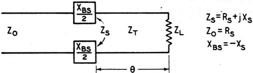
 and
and


 (9)
(9) (10)
(10)

 where W is the rated power
and Z is the characteristic impedance. The voltage at the antenna end of the transformer
section in any of these networks is
where W is the rated power
and Z is the characteristic impedance. The voltage at the antenna end of the transformer
section in any of these networks is
 The voltage at the sending
end of the Q section and the shunt-balanced network is
The voltage at the sending
end of the Q section and the shunt-balanced network is
 In the series-balanced
network it is
In the series-balanced
network it is
 where IL
is the current at the antenna and equal to
where IL
is the current at the antenna and equal to
 When ZL <
Z0 maximum voltage is at the sending end in any of these networks, while
when ZL > Z0 maximum voltage is found at the antenna end.
When ZL <
Z0 maximum voltage is at the sending end in any of these networks, while
when ZL > Z0 maximum voltage is found at the antenna end.

|
||||||||||||||||||||||||||||||||||||