S-, h-, T-, Y-, Z-, ABCD- Parameter Conversions

Conversion formulas between various forms of 2-port network electrical parameters is difficult to find (at least when I first posted these way back in 2001), so once I finally located the paper that included them¹, I felt it was my duty to publish it for public access. The paper is available on the IEEE website by subscribers only. None that I found also include the correction paper² published a year later that addresses some of the technicalities of the S- and T-parameter translations when complex impedance reference planes are used. In order to avoid those sticky issues, I have reproduced only the sets of translations that are unaffected. Many thanks to Mr. Frickey for his unique work.

One of the most sought-after sets of conversion is from s-parameters to T-parameters, and then back to s-parameters. This is because matrix multiplications can be performed directly on T-parameters in order to calculate cascaded component responses. That is, s-parameters matrices cannot be multiplied in series to obtain cascaded s-parameters, but T-parameters can be. So, convert your component s-parameters to T-parameters, multiply matrices, then convert the result back to s-parameters.

The 2-port network shown to the above is representative of what is implied in the application of these equations. Basic relationships of voltage and current are given in the table to the right. Many other sources exist on the particulars of 2-port network analysis, so it will not be covered here.

All of the parameter equations make use of complex values for all numbers of impedance and the resulting matrix parameters, i.e., Z = R ± jX.

Z₀₁ and Z₀₂ are the complex impedances of ports 1 and 2, respectively; similarly, Z*₀₁ and Z*₀₂ are the complex conjugates of the respective impedances.

The values R₀₁ and R₀₂ are the real parts of port impedances Z₀₁ and Z₀₂.

Two RF Cafe visitors, Mr. Louis J. and Mr. Andy H. have written to comment on Fricke's equations.

If you do not already know, here is the meaning of each type of parameter matrix: S (scattering), Y (admittance), Z (impedance), h (hybrid), ABCD (chain), and T (chain scattering or chain transfer).

These are all I have, so please do not write to ask if I have others.

S-Parameters from Z-Parameters
S-Parameters from Y-Parameters
S-Parameters from h-Parameters
S-Parameters from ABCD-Parameters
T-Parameters from Z-Parameters
T-Parameters from Y-Parameters
T-Parameters from h-Parameters
T-Parameters from ABCD-Parameters
Y-Parameters from T-Parameters
Y-Parameters from S-Parameters
Z-Parameters from T-Parameters
h-Parameters from S-Parameters
h-Parameters from T-Parameters (see notes 4 and 5.)
ABCD-Parameters from S-Parameters
ABCD-Parameters from T-Parameters

1. IEEE Transactions on Microwave Theory and Techniques. Vol. 42, No 2. February 1994. Conversions Between S, Z, Y, h, ABCD, and T Parameters which are Valid for Complex Source and Load Impedances. By Dean A. Frickey, Member, IEEE

2. IEEE Transactions on Microwave Theory and Techniques. Vol 43, No 4. April 1995. A correction was printed by Roger B. Marks and Dylan F. Williams.

3. I₁ formula corrected to use V₂ rather than V₁. Thanks to Christoph T. for noticing.

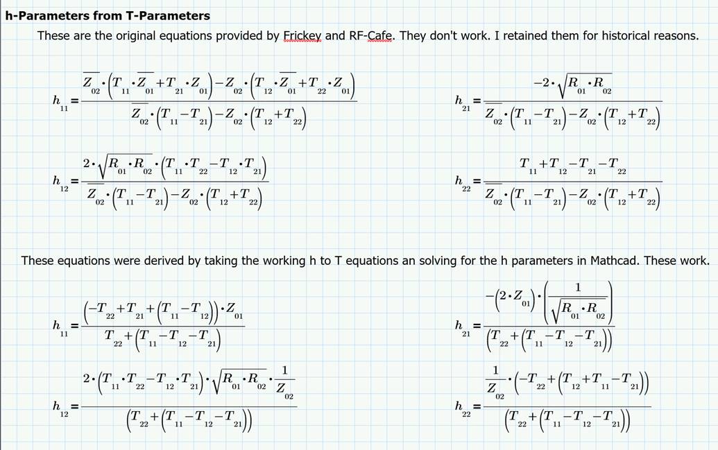
4. Here is Andy H.'s message:

In regards to the page dealing with two port conversions: https://www.rfcafe.com/references/electrical/s-h-y-z.htm. Frickey's original work is indeed correct. I put the equations into Sympy and solved them symbolically to show they match as given below. I also implemented them in Python to numerically show they are correct. Finally, I implemented Louis J.'s version and those only work for real-valued impedances. This is apparent as no components of Z01 or Z02 are ever conjugated in his expressions.

 

import sympy as sp

t11, t12, t21, t22 = sp.symbols('t11, t12, t21, t22') h11, h12, h21, h22 = sp.symbols('h11, h12, h21, h22') z01, z02, z01c, z02c, R = sp.symbols('z01, z02, z01c, z02c, R')

eq1 = sp.Eq(( (-h11-z01) * (1+h22*z02) + h12*h21*z02 ) / (2*h21*R), t11) eq2 = sp.Eq(( (h11+z01) * (1-h22*z02c) + h12*h21*z02c ) / (2*h21*R), t12) eq3 = sp.Eq(( (z01c-h11) * (1+h22*z02) + h12*h21*z02 ) / (2*h21*R), t21) eq4 = sp.Eq(( (h11-z01c) * (1-h22*z02c) + h12*h21*z02c ) / (2*h21*R), t22)

ans = sp.solve((eq1, eq2, eq3, eq4), (h11, h12, h21, h22))

print(ans)

[((t11*z01c*z02c - t12*z01c*z02 + t21*z01*z02c - t22*z01*z02) / (t11*z02c - t12*z02 - t21*z02c + t22*z02),

2*R*(t11*t22 - t12*t21) / (t11*z02c - t12*z02 - t21*z02c + t22*z02),

-(z01 + z01c)*(z02 + z02c) / (2*R*(t11*z02c - t12*z02 - t21*z02c + t22*z02)),

(t11 + t12 - t21 - t22) / (t11*z02c - t12*z02 - t21*z02c + t22*z02))]

----- Comparison with Complex Impedances ----- import numpy as np

def t_to_h_frickey(t, z0):

z0c = np.matrix.conj(z0)

h = np.zeros([2,2], dtype=complex)

denominator = z0c[1] * (t[0,0] - t[1,0]) - z0[1] * (t[0,1] - t[1,1])

h[0,0] = z0c[1]*(t[0,0] * z0c[0] + t[1,0] * z0[0]) - z0[1] * (t[0,1] * z0c[0] + t[1,1] * z0[0]) h[0,1] = 2 * np.sqrt(z0[0].real * z0[1].real) * (t[0,0] * t[1,1] - t[0,1] * t[1,0]) h[1,0] = -2 * np.sqrt(z0[0].real * z0[1].real) h[1,1] = t[0,0] + t[0,1] - t[1,0] - t[1,1]

return h / denominator

def t_to_h_louis(t, z0):

z0c = np.matrix.conj(z0)

h = np.zeros([2,2], dtype=complex)

denominator = t[1,1] + t[0,0] - t[0,1] - t[1,0]

h[0,0] = z0[0] * (-t[1,1] + t[1,0] + t[0,0] - t[0,1]) h[0,1] = 2 * (t[0,0] * t[1,1] - t[0,1] * t[1,0]) * np.sqrt(z0[0].real * z0[1].real) / z0[1] h[1,0] = -2 * z0[0] / np.sqrt(z0[0].real * z0[1].real) h[1,1] = (-t[1,1] + t[0,1] + t[0,0] - t[1,0]) / z0[1]

return h / denominator

def h_to_t(h, z0):

z0c = np.matrix.conj(z0)

t = np.zeros([2,2], dtype=complex)

denominator = 2 * h[1,0] * np.sqrt(z0[0].real * z0[1].real)

t[0,0] = (-h[0,0] - z0[0]) * (1 + h[1,1] * z0[1]) + h[0,1] * h[1,0] * z0[1] t[0,1] = (h[0,0] + z0[0]) * (1 - h[1,1] * z0c[1]) + h[0,1] * h[1,0] * z0c[1] t[1,0] = (z0c[0] - h[0,0]) * (1 + h[1,1] * z0[1]) + h[0,1] * h[1,0] * z0[1] t[1,1] = (h[0,0] - z0c[0]) * (1 - h[1,1] * z0c[1]) + h[0,1] * h[1,0] * z0c[1]

return t / denominator

t11 = 1 + 1j * 2 t12 = 5 - 1j * 8 t21 = -4 + 1j * 3 t22 = 2 + 1j * 1

t = np.array([[t11, t12], [t21, t22]])

# T <--> H z1, z2 = 50 + 10j, 50 - 10j

h = t_to_h_frickey(t, np.array([z1, z2])) print('Frickey:') print(f'Conversion from T to H \n{h}') print(f'Conversion from H to T \n{h_to_t(h, np.array([z1, z2]))}')

h = t_to_h_louis(t, np.array([z1, z2])) print('Louis:') print(f'Conversion from T to H \n{h}') print(f'Conversion from H to T \n{h_to_t(h, np.array([z1, z2]))}')

Frickey: Conversion from T to H [[ 3.90532544e+01+5.62721893e+01j -7.75147929e+00-2.39644970e+00j] [-7.39644970e-02+1.77514793e-01j -1.18343195e-02-2.15976331e-02j]]

Conversion from H to T [[ 1.+2.j 5.-8.j] [-4.+3.j 2.+1.j]]

Louis: Conversion from T to H [[ 4.05882353e+01+8.76470588e+01j -9.43438914e+00-3.41628959e+00j] [-1.05882353e-01+2.23529412e-01j -1.33484163e-02-2.73755656e-02j]]

Conversion from H to T [[ 1. +2.j 5.92307692-661538462j] [-3.61538462+3.92307692j 2.84615385+1.07692308j]]

----- Comparison with Real-Valued Impedances -----

t11 = 1 + 1j * 2 t12 = 5 - 1j * 8 t21 = -4 + 1j * 3 t22 = 2 + 1j * 1

t = np.array([[t11, t12], [t21, t22]])

# T <--> H z1, z2 = 50 + 0j, 50 - 0j

h = t_to_h_frickey(t, np.array([z1, z2])) print('Frickey:') print(f'Conversion from T to H \n{h}') print(f'Conversion from H to T \n{h_to_t(h, np.array([z1, z2]))}')

h = t_to_h_louis(t, np.array([z1, z2])) print('Louis:') print(f'Conversion from T to H \n{h}') print(f'Conversion from H to T \n{h_to_t(h, np.array([z1, z2]))}')

Frickey: Conversion from T to H [[ 5.58823529e+01+7.64705882e+01j -1.01176471e+01-1.52941176e+00j] [-5.88235294e-02+2.35294118e-01j -1.88235294e-02-2.47058824e-02j]] Conversion from H to T [[ 1.+2.j 5.-8.j] [-4.+3.j 2.+1.j]]

Louis: Conversion from T to H [[ 5.58823529e+01+7.64705882e+01j -1.01176471e+01-1.52941176e+00j] [-5.88235294e-02+2.35294118e-01j -1.88235294e-02-2.47058824e-02j]] Conversion from H to T [[ 1.+2.j 5.-8.j] [-4.+3.j 2.+1.j]]

---

Then:

I went down a rabbit hole and programmed (in Python) all of the conversions in the paper, and made test cases that I put in a separate Python file. The test cases use measured data from an Analog Devices HMC455LP3 high output IP3 GaAs InGaP heterojunction bipolar transistor. I have attached both files and I will default to you as to whether or not to post the contents.

---

# IEEE TRANSACTIONS ON MICROWAVE THEORY AND TECHNIQUES. VOL 42, NO 2. FEBRUARY 1994
# Conversions Between S, Z, Y, h, ABCD, and T Parameters which are Valid for Complex Source and Load Impedances
# Dean A. Frickey, Member, EEE

# Tables I and II

import numpy as np
from two_port_conversions import *

""" Testing """
# Analog Devices - HMC455LP3 - S parameters
# High output IP3 GaAs InGaP Heterojunction Bipolar Transistor

# MHz S (Magntidue and Angle (deg))
# 1487.273 0.409 160.117 4.367 163.864 0.063 115.967 0.254 -132.654

s11 = 0.409 * np.exp(1j * np.radians(160.117))
s12 = 4.367 * np.exp(1j * np.radians(163.864))
s21 = 0.063 * np.exp(1j * np.radians(115.967))
s22 = 0.254 * np.exp(1j * np.radians(-132.654))

s_orig = np.array([[s11, s12], [s21, s22]])

# Data specified at 50 Ohms (adding small complex component to test conversions)
z1, z2 = 50 + 0.01j, 50 - 0.02j
z0 = np.array([z1, z2])

""" Conversions """
print(f'Original S: \n{s_orig}\n')

# S --> Z --> T --> Z --> S
z = s_to_z(s_orig, z0)
t = z_to_t(z, z0)
z = t_to_z(t, z0)
s = z_to_s(z, z0)
print(f'Test (S --> Z --> T --> Z --> S): \n{s}\n')

# S --> Y --> T --> Y --> S
y = s_to_y(s_orig, z0)
t = y_to_t(y, z0)
y = t_to_y(t, z0)
s = y_to_s(y, z0)
print(f'Test (S --> Y --> T --> Y --> S): \n{s}\n')

# S --> H --> T --> H --> S
h = s_to_h(s_orig, z0)
t = h_to_t(h, z0)
h = t_to_h(t, z0)
s = h_to_s(h, z0)
print(f'Test (S --> H --> T --> H --> S): \n{s}\n')

# S --> ABCD --> T --> ABCD --> S
abcd = s_to_abcd(s_orig, z0)
t = abcd_to_t(abcd, z0)
abcd = t_to_abcd(t, z0)
s = abcd_to_s(abcd, z0)
print(f'Test (S --> ABCD --> T --> ABCD --> S): \n{s}\n')

 

---

# IEEE TRANSACTIONS ON MICROWAVE THEORY AND TECHNIQUES. VOL 42, NO 2. FEBRUARY 1994
# Conversions Between S, Z, Y, h, ABCD, and T Parameters which are Valid for Complex Source and Load Impedances
# Dean A. Frickey, Member, EEE

# Tables I and II

import numpy as np

def s_to_z(s, z0):
""" Scattering (S) to Impedance (Z)

:param s: The scattering matrix.
:param z0: The port impedances (Ohms).
:return: The impedance matrix.
"""
# Calculate the conjugate of the port impedances
z0c = np.matrix.conj(z0)

# Initialize the output array
z = np.zeros([2,2], dtype=complex)

# Calculate the denominator
denominator = (1 - s[0,0]) * (1 - s[1,1]) - s[0,1] * s[1,0]

# Calculate the numerators
z[0,0] = (z0c[0] + s[0,0] * z0[0]) * (1 - s[1,1]) + s[0,1] * s[1,0] * z0[0]
z[0,1] = 2 * s[0,1] * np.sqrt(z0[0].real * z0[1].real)
z[1,0] = 2 * s[1,0] * np.sqrt(z0[0].real * z0[1].real)
z[1,1] = (1 - s[0,0]) * (z0c[1] + s[1,1] * z0[1]) + s[0,1] * s[1,0] * z0[1]

# Return the conversion
return z / denominator


def z_to_s(z, z0):
""" Impedance (Z) to Scattering (S)

:param z: The impedance matrix.
:param z0: The port impedances (Ohms).
:return: The scattering matrix.
"""
# Calculate the conjugate of the port impedances
z0c = np.matrix.conj(z0)

# Initialize the output array
s = np.zeros([2,2], dtype=complex)

# Calculate the denominator
denominator = (z[0,0] + z0[0]) * (z[1,1] + z0[1]) - z[0,1] * z[1,0]

# Calculate the numerators
s[0,0] = (z[0,0] - z0c[0]) * (z[1,1] + z0[1]) - z[0,1] * z[1,0]
s[0,1] = 2 * z[0,1] * np.sqrt(z0[0].real * z0[1].real)
s[1,0] = 2 * z[1,0] * np.sqrt(z0[0].real * z0[1].real)
s[1,1] = (z[0,0] + z0[0]) * (z[1,1] - z0c[1]) - z[0,1] * z[1,0]

# Return the conversion
return s / denominator


def s_to_y(s, z0):
""" Scattering (S) to Admittance (Y)

:param s: The scattering matrix.
:param z0: The port impedances (Ohms).
:return: The admittance matrix.
"""
# Calculate the conjugate of the port impedances
z0c = np.matrix.conj(z0)

# Initialize the output array
y = np.zeros([2,2], dtype=complex)

# Calculate the denominator
denominator = (z0c[0] + s[0,0] * z0[0]) * (z0c[1] + s[1,1] * z0[1]) - s[0,1] * s[1,0] * z0[0] * z0[1]

# Calculate the numerators
y[0,0] = (1 - s[0,0]) * (z0c[1] + s[1,1] * z0[1]) + s[0,1] * s[1,0] * z0[1]
y[0,1] = -2 * s[0,1] * np.sqrt(z0[0].real * z0[1].real)
y[1,0] = -2 * s[1,0] * np.sqrt(z0[0].real * z0[1].real)
y[1,1] = (z0c[0] + s[0,0] * z0[0]) * (1 - s[1,1]) + s[0,1] * s[1,0] * z0[0]

# Return the conversion
return y / denominator


def y_to_s(y, z0):
""" Admittance (Y) to Scattering (S)

:param y: The admittance matrix.
:param z0: The port impedances (Ohms).
:return: The scattering matrix.
"""
# Calculate the conjugate of the port impedances
z0c = np.matrix.conj(z0)

# Initialize the output array
s = np.zeros([2,2], dtype=complex)

# Calculate the denominator
denominator = (1 + y[0,0] * z0[0]) * (1 + y[1,1] * z0[1]) - y[0,1] * y[1,0] * z0[0] * z0[1]

# Calculate the numerators
s[0,0] = (1 - y[0,0] * z0c[0]) * (1 + y[1,1] * z0[1]) + y[0,1] * y[1,0] * z0c[0] * z0[1]
s[0,1] = -2 * y[0,1] * np.sqrt(z0[0].real * z0[1].real)
s[1,0] = -2 * y[1,0] * np.sqrt(z0[0].real * z0[1].real)
s[1,1] = (1 + y[0,0] * z0[0]) * (1 - y[1,1] * z0c[1]) + y[0,1] * y[1,0] * z0[0] * z0c[1]

# Return the conversion
return s / denominator


def s_to_h(s, z0):
""" Scattering (S) to Hybrid (H)

:param s: The scattering matrix.
:param z0: The port impedances (Ohms).
:return: The hybrid matrix.
"""
# Calculate the conjugate of the port impedances
z0c = np.matrix.conj(z0)

# Initialize the output array
h = np.zeros([2,2], dtype=complex)

# Calculate the denominator
denominator = (1 - s[0,0]) * (z0c[1] + s[1,1] * z0[1]) + s[0,1] * s[1,0] * z0[1]

# Calculate the numerators
h[0,0] = (z0c[0] + s[0,0] * z0[0]) * (z0c[1] + s[1,1] * z0[1]) - s[0,1] * s[1,0] * z0[0] * z0[1]
h[0,1] = 2 * s[0,1] * np.sqrt(z0[0].real * z0[1].real)
h[1,0] = -2 * s[1,0] * np.sqrt(z0[0].real * z0[1].real)
h[1,1] = (1 - s[0,0]) * (1 - s[1,1]) - s[0,1] * s[1,0]

# Return the conversion
return h / denominator


def h_to_s(h, z0):
""" Hybrid (H) to Scattering (S)

:param h: The hybrid matrix.
:param z0: The port impedances (Ohms).
:return: The scattering matrix.
"""
# Calculate the conjugate of the port impedances
z0c = np.matrix.conj(z0)

# Initialize the output array
s = np.zeros([2,2], dtype=complex)

# Calculate the denominator
denominator = (z0[0] + h[0,0]) * (1 + h[1,1] * z0[1]) - h[0,1] * h[1,0] * z0[1]

# Calculate the numerators
s[0,0] = (h[0,0] - z0c[0]) * (1 + h[1,1] * z0[1]) - h[0,1] * h[1,0] * z0[1]
s[0,1] = 2 * h[0,1] * np.sqrt(z0[0].real * z0[1].real)
s[1,0] = -2 * h[1,0] * np.sqrt(z0[0].real * z0[1].real)
s[1,1] = (z0[0] + h[0,0]) * (1 - h[1,1] * z0c[1]) + h[0,1] * h[1,0] * z0c[1]

# Return the conversion
return s / denominator


def s_to_abcd(s, z0):
""" Scattering to Chain (ABCD)

:param s: The scattering matrix.
:param z0: The port impedances (Ohms).
:return: The chain matrix.
"""
# Calculate the conjugate of the port impedances
z0c = np.matrix.conj(z0)

# Initialize the output array
ans = np.zeros([2,2], dtype=complex)

# Calculate the denominator
denominator = 2 * s[1,0] * np.sqrt(z0[0].real * z0[1].real)

# Calculate the numerators
ans[0,0] = (z0c[0] + s[0,0] * z0[0]) * (1 - s[1,1]) + s[0,1] * s[1,0] * z0[0]
ans[0,1] = (z0c[0] + s[0,0] * z0[0]) * (z0c[1] + s[1,1] * z0[1]) - s[0,1] * s[1,0] * z0[0] * z0[1]
ans[1,0] = (1 - s[0,0]) * (1 - s[1,1]) - s[0,1] * s[1,0]
ans[1,1] = (1 - s[0,0]) * (z0c[1] + s[1,1] * z0[1]) + s[0,1] * s[1,0] * z0[1]

# Return the conversion
return ans / denominator


def abcd_to_s(abcd, z0):
""" Chain (ABCD) to Scattering (S)

:param abcd: The chain matrix.
:param z0: The port impedances (Ohms).
:return: The scattering matrix.
"""
# Break out the components
A = abcd[0,0]
B = abcd[0,1]
C = abcd[1,0]
D = abcd[1,1]

# Calculate the conjugate of the port impedances
z0c = np.matrix.conj(z0)

# Initialize the output array
s = np.zeros([2,2], dtype=complex)

# Calculate the denominator
denominator = A * z0[1] + B + C * z0[0] * z0[1] + D * z0[0]

# Calculate the numerators
s[0,0] = A * z0[1] + B - C * z0c[0] * z0[1] - D * z0c[0]
s[0,1] = 2 * (A * D - B * C) * np.sqrt(z0[0].real * z0[1].real)
s[1,0] = 2 * np.sqrt(z0[0].real * z0[1].real)
s[1,1] = -A * z0c[1] + B - C * z0[0] * z0c[1] + D * z0[0]

# Return the conversion
return s / denominator


def t_to_z(t, z0):
""" Chain Transfer (T) to Impedance (Z)

:param t: The chain transfer matrix.
:param z0: The port impedances (Ohms).
:return: The impedance matrix.
"""
# Calculate the conjugate of the port impedances
z0c = np.matrix.conj(z0)

# Initialize the output array
z = np.zeros([2,2], dtype=complex)

# Calculate the denominator
denominator = t[0,0] + t[0,1] - t[1,0] - t[1,1]

# Calculate the numerators
z[0,0] = z0c[0] * (t[0,0] + t[0,1]) + z0[0] * (t[1,0] + t[1,1])
z[0,1] = 2 * np.sqrt(z0[0].real * z0[1].real) * (t[0,0] * t[1,1] - t[0,1] * t[1,0])
z[1,0] = 2 * np.sqrt(z0[0].real * z0[1].real)
z[1,1] = z0c[1] * (t[0,0] - t[1,0]) - z0[1] * (t[0,1] - t[1,1])

# Return the conversion
return z / denominator


def z_to_t(z, z0):
""" Impedance (Z) to Chain Transfer (T)

:param z: The impedance matrix.
:param z0: The port impedances (Ohms).
:return: The chain transfer matrix.
"""
# Calculate the conjugate of the port impedances
z0c = np.matrix.conj(z0)

# Initialize the output array
t = np.zeros([2,2], dtype=complex)

# Calculate the denominator
denominator = 2 * z[1,0] * np.sqrt(z0[0].real * z0[1].real)

# Calculate the numerators
t[0,0] = (z[0,0] + z0[0]) * (z[1,1] + z0[1]) - z[0,1] * z[1,0]
t[0,1] = (z[0,0] + z0[0]) * (z0c[1] - z[1,1]) + z[0,1] * z[1,0]
t[1,0] = (z[0,0] - z0c[0]) * (z[1,1] + z0[1]) - z[0,1] * z[1,0]
t[1,1] = (z0c[0] - z[0,0]) * (z[1,1] - z0c[1]) + z[0,1] * z[1,0]

# Return the conversion
return t / denominator


def t_to_y(t, z0):
""" Chain Transfer (T) to Admittance (Y)

:param t: The chain transfer matrix.
:param z0: The port impedances (Ohms).
:return: The admittance matrix.
"""
# Calculate the conjugate of the port impedances
z0c = np.matrix.conj(z0)

# Initialize the output array
y = np.zeros([2,2], dtype=complex)

# Calculate the denominator
denominator = t[0,0] * z0c[0] * z0c[1] - t[0,1] * z0c[0] * z0[1] + t[1,0] * z0[0] * z0c[1] - t[1,1] * z0[0] * z0[1]

# Calculate the numerators
y[0,0] = z0c[1] * (t[0,0] - t[1,0]) - z0[1] * (t[0,1] - t[1,1])
y[0,1] = -2 * np.sqrt(z0[0].real * z0[1].real) * (t[0,0] * t[1,1] - t[0,1] * t[1,0])
y[1,0] = -2 * np.sqrt(z0[0].real * z0[1].real)
y[1,1] = z0c[0] * (t[0,0] + t[0,1]) + z0[0] * (t[1,0] + t[1,1])

# Return the conversion
return y / denominator


def y_to_t(y, z0):
""" Admittance (Y) to Chain Transfer (T)

:param y: The admittance matrix.
:param z0: The port impedances (Ohms).
:return: The chain transfer matrix.
"""
# Calculate the conjugate of the port impedances
z0c = np.matrix.conj(z0)

# Initialize the output array
t = np.zeros([2,2], dtype=complex)

# Calculate the denominator
denominator = 2 * y[1,0] * np.sqrt(z0[0].real * z0[1].real)

# Calculate the numerators
t[0,0] = (-1 - y[0,0] * z0[0]) * (1 + y[1,1] * z0[1]) + y[0,1] * y[1,0] * z0[0] * z0[1]
t[0,1] = (1 + y[0,0] * z0[0]) * (1 - y[1,1] * z0c[1]) + y[0,1] * y[1,0] * z0[0] * z0c[1]
t[1,0] = (y[0,0] * z0c[0] - 1) * (1 + y[1,1] * z0[1]) - y[0,1] * y[1,0] * z0c[0] * z0[1]
t[1,1] = (1 - y[0,0] * z0c[0]) * (1 - y[1,1] * z0c[1]) - y[0,1] * y[1,0] * z0c[0] * z0c[1]

# Return the conversion
return t / denominator


def t_to_h(t, z0):
""" Chain Transfer (T) to Hybrid (H)

:param t: The chain transfer matrix.
:param z0: The port impedances (Ohms).
:return: The hybrid matrix.
"""
# Calculate the conjugate of the port impedances
z0c = np.matrix.conj(z0)

# Initialize the output array
h = np.zeros([2,2], dtype=complex)

# Calculate the denominator
denominator = z0c[1] * (t[0,0] - t[1,0]) - z0[1] * (t[0,1] - t[1,1])

# Calculate the numerators
h[0,0] = z0c[1]*(t[0,0] * z0c[0] + t[1,0] * z0[0]) - z0[1] * (t[0,1] * z0c[0] + t[1,1] * z0[0])
h[0,1] = 2 * np.sqrt(z0[0].real * z0[1].real) * (t[0,0] * t[1,1] - t[0,1] * t[1,0])
h[1,0] = -2 * np.sqrt(z0[0].real * z0[1].real)
h[1,1] = t[0,0] + t[0,1] - t[1,0] - t[1,1]

# Return the conversion
return h / denominator


def h_to_t(h, z0):
""" Hybrid (H) to Chain Transfer (T)

:param t: The hybrid matrix.
:param z0: The port impedances (Ohms).
:return: The chain transfer matrix.
"""
# Calculate the conjugate of the port impedances
z0c = np.matrix.conj(z0)

# Initialize the output array
t = np.zeros([2,2], dtype=complex)

# Calculate the denominator
denominator = 2 * h[1,0] * np.sqrt(z0[0].real * z0[1].real)

# Calculate the numerators
t[0,0] = (-h[0,0] - z0[0]) * (1 + h[1,1] * z0[1]) + h[0,1] * h[1,0] * z0[1]
t[0,1] = (h[0,0] + z0[0]) * (1 - h[1,1] * z0c[1]) + h[0,1] * h[1,0] * z0c[1]
t[1,0] = (z0c[0] - h[0,0]) * (1 + h[1,1] * z0[1]) + h[0,1] * h[1,0] * z0[1]
t[1,1] = (h[0,0] - z0c[0]) * (1 - h[1,1] * z0c[1]) + h[0,1] * h[1,0] * z0c[1]

# Return the conversion
return t / denominator


def t_to_abcd(t, z0):
""" Chain Transfer (T) to Chain (ABCD)

:param t: The chain transfer matrix.
:param z0: The port impedances (Ohms).
:return: The chain matrix.
"""
# Calculate the conjugate of the port impedances
z0c = np.matrix.conj(z0)

# Initialize the output array
ans = np.zeros([2,2], dtype=complex)

# Calculate the denominator
denominator = 2 * np.sqrt(z0[0].real * z0[1].real)

# Calculate the numerators
ans[0,0] = z0c[0] * (t[0,0] + t[0,1]) + z0[0] * (t[1,0] + t[1,1])
ans[0,1] = z0c[1] * (t[0,0] * z0c[0] + t[1,0] * z0[0]) - z0[1] * (t[0,1] * z0c[0] + t[1,1] * z0[0])
ans[1,0] = t[0,0] + t[0,1] - t[1,0] - t[1,1]
ans[1,1] = z0c[1] * (t[0,0] - t[1,0]) - z0[1] * (t[0,1] - t[1,1])

# Return the conversion
return ans / denominator


def abcd_to_t(abcd, z0):
""" Chain (ABCD) to Chain Transfer (T)

:param abcd: The chain matrix.
:param z0: The port impedances (Ohms).
:return: The chain transfer matrix.
"""
# Break out the components
A = abcd[0,0]
B = abcd[0,1]
C = abcd[1,0]
D = abcd[1,1]

# Calculate the conjugate of the port impedances
z0c = np.matrix.conj(z0)

# Initialize the output array
t = np.zeros([2,2], dtype=complex)

# Calculate the denominator
denominator = 2 * np.sqrt(z0[0].real * z0[1].real)

# Calculate the numerators
t[0,0] = A * z0[1] + B + C * z0[0] * z0[1] + D * z0[0]
t[0,1] = A * z0c[1] - B + C * z0[0] * z0c[1] - D * z0[0]
t[1,0] = A * z0[1] + B - C * z0c[0] * z0[1] - D * z0c[0]
t[1,1] = A * z0c[1] - B - C * z0c[0] * z0c[1] + D * z0c[0]

# Return the conversion
return t / denominator

 

5. Here is Louis J.'s message:

h- from T-parameter equations.

Here is Louis' Mathcad file containing all of Frickey's equations.

I'm writing in regard to your S-, h-, T-, Y-, Z-, ABCD- Parameter Conversions web page in which I found three errors.

I was building up a library of Frickey's transforms with the corrections and used your website as a check. I verified all equations could "close the loop" by restoring the original data after going through a pair of related equations or more. Example: S to A to T to Z and back to S. I also verified the intermediate results against other tools that perform the same calculations, including those on line. In this manner, I found the errors in your website, and also in Frickey's work.

Error 1: The equations under the title Y-Parameters from Z-Parameters are not related to the title. They are actually Y from T parameters. This is confirmed by comparing equations in Frickey's document as well as failure to "close the loop".

Error 2: The equation for Z-Parameters from T-Parameters, index 22, is in error. In the numerator is the term Z[02]*(T[12]+T[22]). The addition is actually a subtraction. This is verified both in Frickey's document as well as failure to "close the loop".

Error 3: This is a bug in Frickey's document and you are unlikely to be able to do anything about it. The h-Parameters from T-Parameters equation set fail to close the loop. All four equations have an error that is in the same direction and of roughly the same magnitude as measured in percentage. I suspect a problem with the denominator value. I verified this assumption by adding in an offset (complex) into the denominator and found all values fell into place. Without this offset, these simply refused to "close the loop" or match the results from other tools. I am far from a mathematician, so I tend to rely on Mathcad to do my algebra, trig and calculus. I started with the working T from h parameter equation set. It handled this matrix equation system fairly easily, but didn't provide a common denominator for the four members. I fudged by taking a term from the denominator of three equations and placing the reciprocal in the numerator so the denominators remain common. Mathcad also doesn't include complex conjugates in it's solutions, although it understands them in original equations. As a result, the equations I'm providing are likely sub-optimal.

I have included a screen shot from Mathcad to show my solution.

I don't know how to contact Frickey to inform him of this error. What bothers me is that this document has been in the wild for many years. Why hasn't this been discovered before?

If you use Mathcad, I will happily send you my worksheets and you can play with these equations using live numbers and "closing the loop". This should satisfy you that I'm not blowing smoke.

Thanks for the good work and all the things you place on your website. While I'm not an RF engineer, I use your website regularly while working high speed communication links (28Gb SERDES) and other signal classes having fast rise and fall times (harmonics) and sometimes very high frequency fundamentals.

I stumbled across this document from NASA you may also find of interest. It appears the rebuttal to Frickey's work was itself rebutted by none other than NASA itself. Its amusing reading. Frickey's work still stands as the best reference out there. I don't understand the failure of that one link (T to h), but I've had a couple other engineers up here check my work and they too are satisfied Frickey's T to h equations are broken.

Update with Mathcad File:

Attached is the Mathcad worksheet containing all of Frickey's work, both what you published and what the original paper included that you did not publish.

It does not contain the "close the loop" testing I performed, but all the equations are identical to the ones in my test sheet.

The equations are all configured for symbolic manipulation. To use with live data, copy the equation(s) of interest to another worksheet, change the <ctrl>= to a <colon>= and define the variables. This is something any Mathcad user should know how to do.

Tip: If one were interested, they could copy the content of any equation object in Mathcad (not the equation object itself) and paste it into a generic text editor. The result is an equation using Mathcad functions in RPN format. (Lots of parens so each operation has one or two variables. Each operation consists of the operator followed by the one or two variables. Mathcad functions are preceded by an '@' symbol and are self explanatory.) They can then move it to any tool they want after converting it to the appropriate format. I frequently do this to get equations into Excel.

Posted July 25, 2023
(updated from original post on 2/16/2001)