Magnetism Part I - A Modern View of Permanent Magnet Theory, October 1947 Radio-Craft

This first installment in a multi-part series on magnetism appeared in the October 1947 issue of Radio-Craft magazine. At the time, there was great interest in magnetic tape and even magnetic wire recorders. Lots of articles were published on the electronics and mechanics of recorders, but relatively few discussed the physics of magnetics. Although the title says it is about permanent magnetic theory, there is also a lot of information on electromagnets. Terms such as reluctivity, magnetomotive force, magnetic flux, conductivity of electrical and magnetic circuits, conductance, B-H curves, maxwells, oersteds, and gilberts are introduced, along with some simple equations relating everything. Part II, "Benefits of Tape Recording," appeared in the November 1947 issue and Part III, "Magnetic Recording - Recorder Design," appeared in the December 1947 issue.

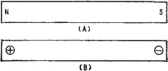
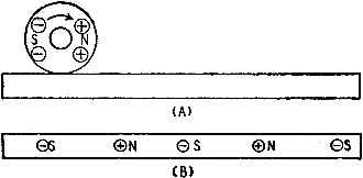
Illustrating the new magnet markings - RF Cafe

Fig. 1 - Illustrating the new magnet markings.

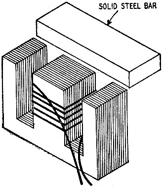
Fig. 2 - Simple equipment for magnet studies.

The subject of magnetism is very old (the compass appears to have been invented over 4,000 years ago), yet it remains one of the least understood of phenomena. It was not until the twelfth century A.D. that European scholars tried to fathom its secrets, though the magnet or lodestone had been known to them for centuries, and mention of it is found in legends dating several centuries B.C.

In Europe as in Asia the magnet found its almost exclusive use as a means for determining direction. This unfortunately caused its poles to be given geographical names (north and south). This clumsy terminology has been an obstacle to the student. We will therefore rename the poles arbitrarily, calling the north (N) pole the positive pole and the south (S) pole the negative pole. To avoid confusion with electrical signs, magnetic pole signs will be circled in drawings, as shown in Fig. 1, and put inside parenthesis in text. This is one of a few new concepts we will introduce in an attempt to present magnetic phenomena more clearly to technicians and experimenters who may be interested in contributing to the art of magnetic recording.

Probably nearly every reader (including the author) was first introduced to the mysteries of magnetism via the old familiar bar magnet. When, in 1820, Sir Humphry Davy magnetized a bit of soft iron by running a current of electricity around it, he produced the first bar electromagnet. For an unobstructed understanding of magnetic recording it is suggested that the reader temporarily forget Davy's bar magnet and how it was made. To help forget, try this experiment:

7. Examine the polarity of this bar magnet with a compass and by sprinkling powdered iron on a sheet of paper placed over the magnet.

Fig. 3 - Two types of permanent magnet fields.

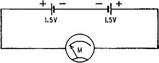
Electric analog of multipole magnet - RF Cafe

Fig. 4 - Electric analog of multipole magnet.

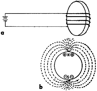
Circuit. for making a disc magnet - RF Cafe

Fig. 5-a - Circuit. for making a disc magnet. 5-b - Chart of disc magnet's force field.

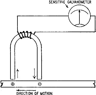
Magnetization of a strip of steel - RF Cafe

Fig. 6 - Magnetization of a strip of steel.

Your examination will show that you have made a magnet with like poles at both ends! The powdered-iron pattern will look like Fig. 3-b instead of the usual magnetic field pattern of Fig. 3-a.

This unusual type of magnet is one of the cornerstones of modern magnetic recording processes.

2. Its polarity resembles that of 2 common bar magnets which have been physically joined at like poles.

If this twin magnet be bent into the familiar horseshoe form, it will not exhibit usual magnetic properties at its terminal poles.

This magnetic characteristic resembles the effect produced by connecting 2 similar batteries back to back and measuring "no voltage" across their outermost terminals (Fig. 4).

If we should pass some current around the flat surfaces of a hard steel disc (Fig. 5-a) about 1 inch in diameter and 1/4 inch thick, we would have a short cylinder magnetized in the direction of its diameter (Fig. 5-b). (You should have forgotten about ordinary bar magnets by now.) If a hole is drilled through its center, a shaft inserted and the wheel rolled on a small hard steel rod or rail (Fig. 6), the rail will become weakly magnetized at the points of polar contact. This passage of magnetic induction from one magnet into a magnetizable substance by contact (or near contact) and the retention of the magnetism by the latter is known as transference. Susceptibility to transference determines the degree of interference to be expected when a turn of magnetically recorded wire comes in direct contact with an adjacent wire.

We now have a rail (a magnetic signal carrier) which has been magnetized (modulated by a magneto-mechanical modulator). We can expose or view (detect) these magnetic modulations in a number of ways. A small compass may be used to explore the magnetic field around the rail; or finely powdered iron may be sprinkled on the rail to find its magnetic nodes; an electro-magnetic detector (a soft iron horse-shoe-shaped rod which passes through a multi-turn coil connected to a sensitive galvanometer and whose ends are separated by a distance equal to half the circumference of the magnetic disc), as illustrated in Fig. 7 may be moved along, and in contact with, the rail; or the rail may be moved against the detector. In any case a voltage will be produced in the coil and indicated by the galvanometer.

This electromagnetic detection process may be reversed by applying a variable voltage to the coil while the carrier (rail) is moved laterally. The rail will be magnetically modulated as suggested in Fig. 2.

We now have covered the 3 basic elements required to record or transmit intelligence via magnetic media:

As the construction, application, and operation of these basic elements play indispensable roles in the final processes of magnetic recording it becomes important to be able to design these elements for optimum performance. Since they are all primarily magnetic devices, designing them naturally calls for the use of magnetic terms. It is therefore important for a full understanding of the process, to become familiar with applicable magnetic terminology, bearing in mind the very special applications to which it will be applied.

Familiarity with academic magnetic terms may be gained by referring to one of a number of text books on magnetism. (Also see "Coils, Cores and Mag-nets" Radio-Craft, October and November, 1946.) For the radio technician and experimenter, it may be easier to understand magnetic phenomena by referring frequently to electrical analogies.

Interpretation of technical descriptions requires an understanding of carefully chosen units and standards to which the names of famous scientists have been applied (for example, fundamental electrical units were named after scientists like Count Alessandro Volta, Georg Simon Ohm, Andre Marie Ampere, James Watt, and others).

Simple magnetic modulation detector - RF Cafe

Fig. 7 - Simple magnetic modulation detector.

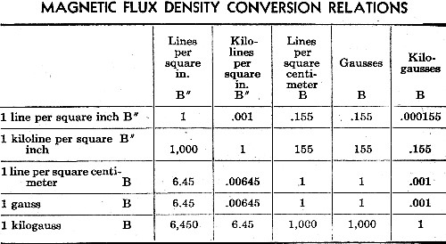
Table I - Magnetic Flux Density Conversion Relations

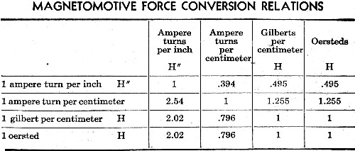
Table II - Magnetomotive Force Conversion Relations

The fundamental units of and formulas relating to magnetic phenomena as developed by physicists are usually expressed in the metric (also called the centimeter-gram-second or c.g.s) system, which has been internationally employed. Interpretation and application of this information is made difficult for English-speaking students accustomed to the clumsier, inch-ounce-second or foot-pound-hour system. Conversion into standard English units are helpful. See Tables I and II.

In magnetics, as in other physical sciences, a fundamental force - Gilbert (after William Gilbert) - is required to produce a quantity - Maxwell (after James Clerk Maxwell) - in a given medium. The ability of the medium to help or hinder the flow of the quantity determines its reluctivity (magnetic resistance) or permeability (magnetic conductance).

Where Where R = resistance in R = reluctivity, ohms, H = magneto- E = electromotive motive force force in volts, in oersteds, I = current in B = magnetic flux amperes. in gauss. Similarly, the conductivity of electrical and magnetic circuits may be approximately compared as follows:

When the force Gilbert is simply related to lineal length of the magnetic circuit (1 Gilbert per centimeter), we have a unit of magnetizing force per unit of length called an oersted (after Hans Christian Oersted). Similarly, when the quantity maxwell is simply related to cross-sectional area (1 maxwell per square centimeter), we have a unit of magnetic quantity-per unit of area - a gauss (after Karl F. Gauss).

The familiar Ohm's Law of electricity now can be compared with its magnetic' equivalent as follows:

Similarly, the conductivity of electrical and magnetic circuits may be approximately compared as follows:

Although many factors are to be considered in the design and manufacture of magnetic tapes or wires for recording purposes, the most important are the residual induction and coercive force of the material. These 2 characteristics are best understood by examining the material's so-called hysteresis loop (which is nothing more than a visual indication of the lagging of magnetic induction - flux - behind the magnetizing force which produces the magnetism in the material), See Fig. 8.

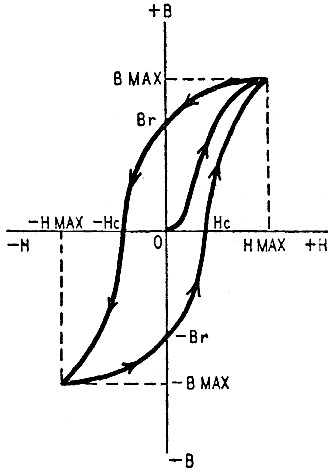
Fig. 8 - Magnetic hysteresis, or B-H curve.

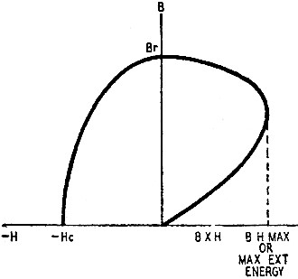
The important demagnetization loop - RF Cafe

Fig. 9 - The important demagnetization loop.

atterns with large gap - RF Cafe

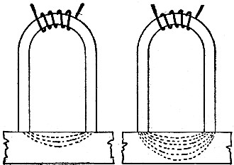
Figs. 10-a and 10-b - Patterns with large gap.

Same signals, smaller gap - RF Cafe

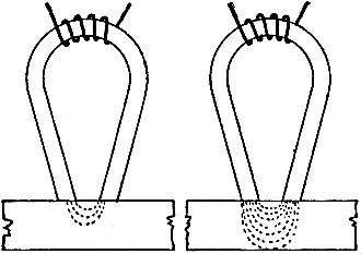
Figs. 10-c. 10-d - Same signals, smaller gap.

The horizontal axis H represents the value of the magnetizing force per unit length applied - positive and negative. The vertical axis B represents the amount of flux per unit area induced in the material. Measurement begins with the material completely demagnetized (at 0 intersection of lines H and B). The magnetizing force is increased to a positive value beyond which further increases in magnetizing force produce no increase in the magnetism of the material. This registers a curve from 0 to B max on the chart. Then the magnetizing force is reduced to zero. However, a certain amount of induced magnetism remains in the material - as represented by the intersection of the return curve from B max to B at Br. This Br value represents the peak residual magnetism the material will retain without demagnetizing influence. From this point, the magnetizing force is changed in direction and increased to a negative saturation. This describes a curve from Br to an intersection with the H line at - Hc and on to a negative B max. Again the magnetizing force is reduced to zero, producing the curve from negative B max to negative Br. Re-establishment of positive magnetizing force carries the curve from negative Br to positive B max. Repetition of this magnetization and demagnetization process will result in the establishment of the complete symmetric loop about point 0 - the hysteresis loop.

Most of the information required about a material is gained in the segment of the hysteresis loop (Br to Hc) known as the demagnetization curve (Fig. 9). As explained, the value marked on the B line at point Br indicates the maximum residual induction. The value marked on the negative side of the H line at Hc indicates the demagnetization force per unit length required to reduce the residual magnetism to zero. This is known as the coercive force of the material. Furthermore, it can be shown that the product of the flux density B and the unit demagnetizing force H represents the amount of magnetic energy that each cubic centimeter of the material is capable of supplying. In actual units, B x H divided by 8 π equals ergs per cubic centimeter. In normal practice, however, only the product of B x H is quoted.

The variation of B x H between Br and Hc is shown on the right side of the demagnetization curve. From a practical standpoint, it can be shown that a magnetic wire or tape designed to operate at a point on the demagnetization curve corresponding to the maximum value of B x H will supply the maximum amount of flux per unit volume of the material.

Other important characteristics of magnetic signal carriers include factors which influence transference, penetration, and self-demagnetization.

Transference, as previously indicated, is the property of transferring magnetic induction from one magnet to another by contact or near-contact. The degree of transference depends upon the magnetomotive force exerted by the modulator, the depth of magnetic penetration, and subsequent self-demagnetization. Both of the latter functions are dependent upon the thickness of the carrier, the air gap in the modulator, and the recorded wave length.

If we could stop the magnetic modulating process instantaneously and examine the magnetic fields produced within the carrier during the peak energy transfer period of a weak and strong signal fed into 2 modulators, one with a relatively large gap and the other with a smaller one, the magnetic field within the carrier probably would resemble Fig. 10.

Fig. 10-a shows the small degree of penetration obtained with a large gap and low signal (magnetomotive energy). Fig. 10-b indicates the deeper penetration obtained with a larger signal. A further increase of signal energy would saturate the carrier. Fig. 10-c shows the shorter effective magnetic field generated in the carrier by the small gap. As the gaps become smaller and smaller the induced magnetic fields become shorter and shorter until the magnetic isolation between pole pieces decreases to a point where a magnetic short takes place so that no energy is subsequently available for excitation of the magnetic detector. This is a form of self-demagnetization. This is roughly equivalent to decreasing the insulation between plates of a condenser until the leakage becomes so high that virtually no charge remains in the condenser. Self-discharge in an electrical sense is approximately analogous to self-demagnetization in a magnetic sense).

Other factors which influence the design and application of magnetic modulators (recording heads), magnetic detectors (playback heads), magnetic demodulators (obliterating heads), and their interrelation with the magnetic carrier (wire or ribbon) will be discussed in a succeeding article Elements of Magnetic Recording scheduled to appear in the November issue of Radio-Craft.

Comments from readers will be welcomed by the author. Address all correspondence care of Radio-Craft.

Magnetism Part I - A Modern View of Permanent Magnet TheoryOctober 1947 Radio-Craft

Magnetism Part I - A Modern View of Permanent Magnet Theory
October 1947 Radio-Craft