Theory and Application of UHF (Part 8) |
||
This is part 8 of an 11-part series authored by Mr. Milton S. Kiver entitled, "Theory and Applications of UHF," that appeared in Radio News magazine in the mid 1940s. As you might expect it is a very extensive delve into the relatively new realm of ultra high frequency (UHF) generation, transmission, propagation, and reception. You might not know that up through the 1930s, UHF circuit and practice had been relegated to the amateur radio operators because those frequencies from 300 MHz to 3 GHz were considered too unexploitable for professional use. It was not until Hams did the hard work of figuring out practical methods of building circuits and antennas and characterizing geographical and atmospheric conditions that affected propagation that suddenly industry and government decided UHF might be useful after all. At that point the Federal Communications Commission (Federal Radio Commission prior to 1934) quickly reallocated spectrum to facilitate its newfound love for the world above 300 MHz. Radio's essential role in World War II was made possible in large part by UHF technology, which includes radar systems. Eleven installments appeared in the following issues: Part 1: December 1943 (p35), 2: January 1944 (p32), 3: March 1944 (p41), 4: April 1944 (p46), 5: May 1944 (p50), 6: August 1944 (p53), 7: October 1944 (p58), 8: December 1944 (56), 8: February 1945 (p58), 10: April 1945 (p57), 11: June 1945 (p57). I hope to eventually procure those editions and post the articles. Theory and Application of UHF By Milton S. Kiver Part 8. The theory and application of cavity resonators as tuning units of Klystron and Magnetron oscillators, operating at u.h.f.
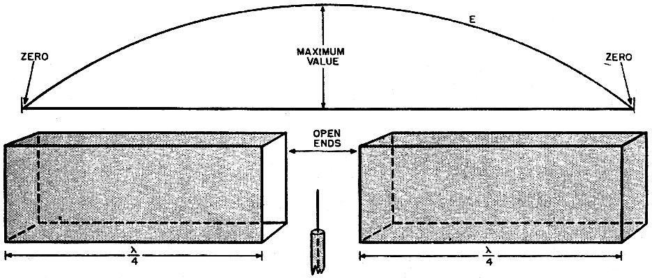
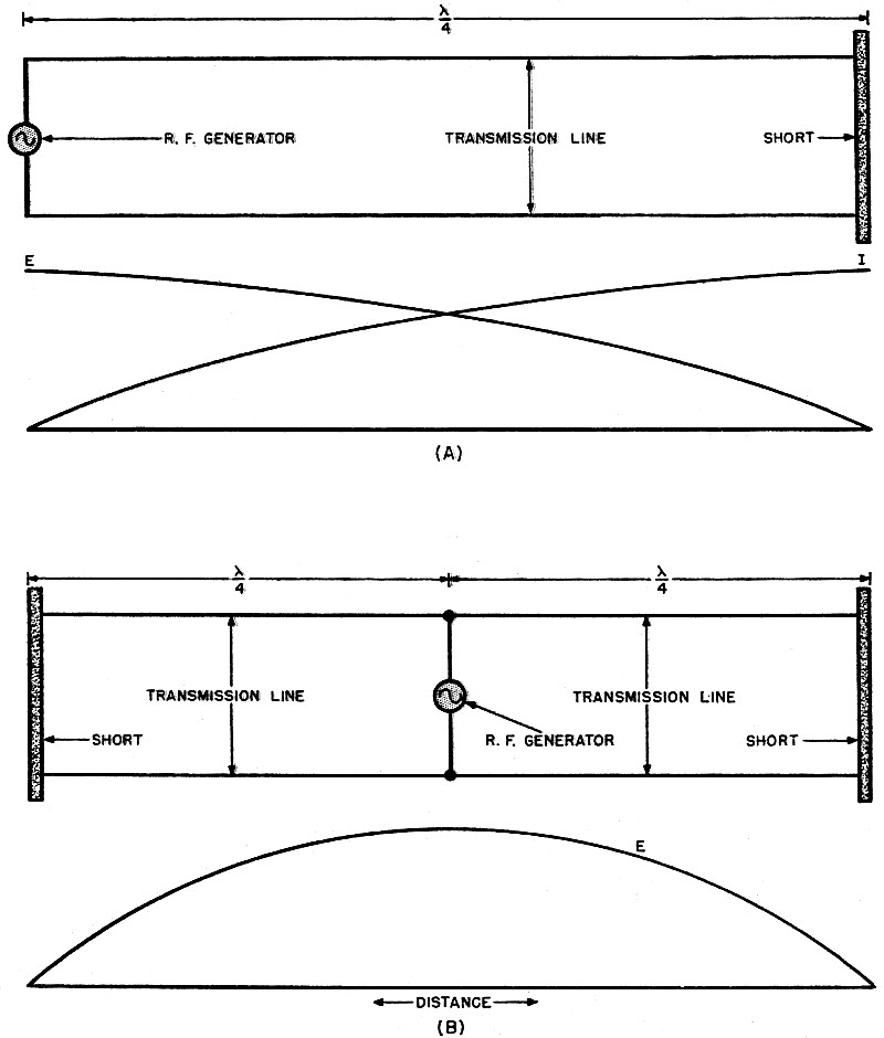
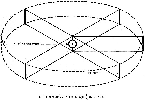
Fig. 1 - (A) Cavity resonator, showing the electric field distribution along the X axis. (B) the same resonator as in (A), showing how the electric field varies as the wave travels down the enclosure. It has been noted in previous articles that the trend in tuning apparatus was from lumped circuit elements at the low frequencies to distributed elements at the ultra-highs. The necessity for using lines arose from the fact that at the wavelengths generated by the Klystron and Magnetron, the size of coils and condensers would have been too small to be of any use. Also, the Q of these circuits would have been very low, not at all comparable to what can be obtained from resonant lines. Now, as the frequency is raised to 3,000 megacycles, even the length of tuned lines becomes a little impractical to use. For example, a quarter-wave line at a wavelength of 10 centimeters is only 2.5 cms. long or roughly one inch. A transmission line this long would be very critical to adjust and we would end up finally with the same sort of situation that occurred with regular tuning coils and condensers. Thus, the time was ripe for modifications of the existing equipment which, it was hoped, would lead to more efficient means of solving this problem, The result of further experimentation led to the development of the cavity resonator which, if you recall, was mentioned as the tuning device on the Klystron oscillator discussed in Part 2. It is the purpose of this article to investigate this new tuning device and see just how its properties stand up against the resonant circuits that preceded it. There are two possible means whereby cavity resonators may be explained. One deals with tuned lines, which is derived from conventional ideas on electric current flow, while the other uses the wave guide as the basis. It might be instructive to analyze each method since it is believed that a better insight into cavity resonators will be attained in this way. To start with the tuned transmission line, consider the quarter-wave section shown in Fig. 6(A). If a generator is coupled to it, then the familiar voltage and current distribution shown will be obtained. (The circuit is being reproduced here for convenience.) At the shorted end of the line, the current will be a maximum and the voltage value will be zero or at least very low. At the open end the reverse will take place resulting in low current and high voltage. These are the conditions that must exist if this line is to operate as a resonant circuit. Now suppose that it is desired to excite two of these quarter-wave lines instead of one. Then they could be placed in parallel across the generator as shown in Fig. 6(B). This combination would now have a higher resonant frequency because essentially the inductances in each line are being placed in parallel with each other, and like resistances in a similar situation, the end result is smaller than any of the components. Continuing this process would result finally in a container having a shape such as shown in Fig. 7. At the center would still be the generator exciting all the infinite number of units that now have been blended into one. This, then, is the final product - the cavity resonator. It might be mentioned that in this process the capacitance has changed very little. In the Klystron oscillator, instead of actually having a generator at the center of this cavity resonator, it will be recalled that holes or openings were made at the center and then bunches of electrons were sent through and these excited the cavity resonator and started its operation. But whether an actual generator is located at the center of the cavity resonator or bunched electrons are sent through, the end result is the' same, namely, excitation of the resonator.
Fig. 2 - A quarter-wave section of a wave guide used to set up standing values of electric and magnetic fields.
Fig. 3 - By using two quarter-wave sections of wave guides, a closed cavity resonator may be had. The above curve gives the electric field distribution inside the guides. The reader will note, at this point, that the electron itself assumes greater importance at the ultra-highs than at the lower frequencies. This does not arise because the electron has different functions at the shorter wavelengths, because it has not. Rather, it is due to the fact that the phenomena can be explained more easily when the individual electron and its effect are considered. Thus, from the above analysis, it may be argued that the cavity resonator is essentially the same as the former quarter-wave tuning lines placed in parallel except that this process was carried to the limit. Remember the voltage distribution on the quarter-wave line as shown in Fig. 6(A), for this will help tie in the cavity as obtained by the above process to that resonator which will be derived now from a waveguide analysis. The easiest way to begin this is to deal with a small section of waveguide, such as pictured in Fig. 2. One end of the waveguide has been blocked and the other end left open so that by means of a small antenna waves can be sent down the guide. These waves will travel unmolested until the end that has been closed is reached. Upon striking this solid wall, a reflection of energy will take place whereupon there will be waves travelling now in two directions, something quite similar to the situation on a transmission line when a change occurs along its length. In order to have the reflected waves reach the opening and arrive there so as to reinforce the electric field previously set up, the end-blocking wall may be made movable and adjusted so that this reinforcement does take place. Standing values of electric and magnetic fields are now set up and this situation is very similar to the quarter-wave tuning line. To complete the above picture, take another such section of a wave guide and place it on the other side of the transmitting antenna as shown in Fig. 3. Waves from the antenna will travel in both directions away from the radiator and both will be reflected when they strike the two closed ends. If the lengths of both guides are equal and correctly adjusted, then the standing waves set up will reinforce at the center and a continuous pattern will be obtained. This is also shown in Fig. 3. By placing the open ends of the sections together, a cavity resonator is the result. Naturally there is only one fundamental frequency that will give the correct electric field distribution as described above. However, by means of other frequencies that are integral multiples (harmonics) of this fundamental, a full wave, a wave and a half, etc., can be placed into the same space. More about this will follow. Meanwhile the reader should notice the marked resemblance between the standing values of electric-field and magnetic-field distribution here with the standing waves of voltage and current encountered on transmission lines under similar conditions. Thus, both methods of deriving cavity resonators are very much alike and it may begin to dawn upon the reader that although it has not been specifically mentioned before, the waveguide (and hence the cavity resonator) may be considered as a transmission line carried to the limit. The relationship between voltages and currents and electric and magnetic fields will be more fully explained in a later article. From the foregoing discussion it is possible to arrive at the minimum length that a cavity resonator must possess in order to function properly at some given frequency. They should be at least a half wave in length. This fact can be understood quite simply, for it will be remembered that in order to derive a resonator, the distance from one end of one waveguide section to the generator was 1/4 wavelength. To go on from the generator to the opposite end of the other wave guide section meant another 1/4 wavelength, giving the sum total of 1/2 wavelength. Naturally, if one 1/2-wavelength cavity resonator will work, so will a resonator that is any whole number multiple, such as a full wavelength, one and a half, etc. This same sort of situation holds true when considering ordinary transmitting antennas where a half-wave Hertz, a full-wave Hertz or any multiple of a half-wave antenna will work. The basic principle remains the same. The object in having the length of the resonator exactly an integral (or whole number) multiple of the first half-wave unit is quite obvious. Any wave sent out, say from the antenna, must be reflected and returned so that the maximum amplitude or strength of the standing wave is obtained. This will occur for only one distance or, as stated above, multiples of this distance. The minute any change occurs in the distance, the forward and backward (or reflected) waves no longer will act so as to aid each other and weak standing waves will be set up, resulting in inefficient operation of the resonator as a tuning unit. The distance from the antenna (or generator) to where the wave is reflected is quite sharp and must always be adjusted carefully. Now that the length of a cavity resonator has been determined, it would be best to investigate the distribution of the magnetic and electric fields in a resonator. This will prove helpful when methods for extracting the energy from a resonator are considered. An investigation of the way the electric and magnetic fields are distributed in a cavity resonator should not be too complicated if the facts mentioned in the chapter on wave guides are remembered. It was here that the various wave intensities were shown and explained for waveguides and, as just pointed out, a cavity resonator may be considered as essentially derived from a waveguide. To begin, consider the small rectangular cavity resonator shown in Fig. 1(A). Any electric wave set up must be so arranged that at any of the walls its intensity will be zero. If this condition is not adhered to, then currents due to this electric field will flow at these boundaries and distort the whole waveform. This specification was likewise demanded in the waveguide. In order to satisfy this condition, a wave will be set up across dimension X (the width of this rectangular box) so that it is maximum in the center and gradually tapers off to zero at the sides. This is also illustrated in the above figure.
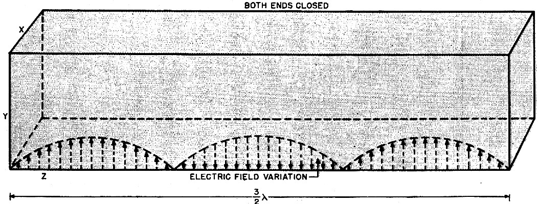
Fig. 4 - An example of a cavity resonator one and one-half wavelengths long. The arrows represent the directions of the electric field set up within the resonator.
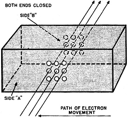
Fig. 5 - By allowing electrons to pass through the cavity resonator, it is possible to excite the resonator and cause large values of electric and magnetic fields to be formed.
Fig. 6 - (A) The familiar 1/4·wave transmission line, showing its voltage and current standing waves. (B) Two 1/4-wave lines in parallel across one generator. The next point in the electric field distribution to consider will be the length of this cavity resonator, the dimension Z in Fig. 1(B), A three-dimensional picture is being dealt with here so that not only will the electric field vary along the X axis as mentioned above, but it will also change as it moves down the length of this enclosure. And as the wave travels down the length of the resonator, it must reach the end wall of the resonator so that its electric field is again zero. This is depicted separately in Fig. 1(B) and the length of the resonator has been adjusted so that it is one half-wave long. Thus, if the three-dimensional picture is to be visualized, there would be a half-wave variation in electric-field intensity along dimension X and one half-wave distribution along Z. To illustrate another situation, see Fig. 4, where the electric-field intensity along the X axis is still the same, but now the length is longer and there is a full wave and a half distance. No matter how long or wide these resonators may be, even in different forms, the rules as laid down in previous articles regarding the distributions of electric and magnetic fields still hold. This explanation has dealt exclusively with electric fields, but of course there are magnetic fields present also. These have been omitted purposely in order to simplify this discussion, else a complicated diagram drawn in three dimensions would have been necessary to obtain the desired effect. For the present it is merely necessary to remember that the fields are at right angles to each other. And, as in wave guides or just plain electromagnetic waves in space, the r.f. energy oscillates between the magnetic and electric fields. One instant it is in the electric field, the next it has smoothly changed over to the magnetic field. The rate at which the changes occur is the same as the frequency of the wave itself. And, as pointed out before, it is through this interchange of energy that the wave sustains itself and moves forward. Whether in a cavity resonator, a wave guide, or just in ordinary space, the same things happen in the exact same manner. The only differences refer to the minor restrictions imposed by the confining walls of the enclosure. The above resonator was excited by an antenna placed inside the box. For some applications of these devices, this is the method used. But there are many more places where electrons are the exciting agency. To understand this method of operation, consider the chamber shown in Fig. 5. This is similar to the other cavity resonators described above, except that the sides have been altered slightly. Now at the center of the sides a series of holes have been drilled so as to allow the passage of a stream of electrons through the center of the resonator. Every time an electron approaches side A, there is a movement or displacement of negative electrons away from this side, repelled, of course, by the charge on the approaching electron. As this electron swings through the openings in the resonator itself, the induced positive charge may be thought as moving with it, only this positive charge is confined to the surface of the metal. When the electron leaves the resonator through side B, the electric charge that it induced may be considered as released and now it moves back to its starting point. Thus, there is a flow of current in one direction when the electron passes through and a flow in the opposite direction when the induced charge returns to its previous rest position. This may be compared to a pendulum that is pushed aside every time something passes it and then returns to its former position when the disturbance has gone. In both cases oscillations will occur, which is the desired effect in the cavity resonator. If the exciting electrons swing through the cavity resonator at definite times, then the oscillations set up in the resonator will continue just as in the case of an ordinary oscillating circuit. Needless to say, the definite frequency mentioned in the last statement must bear a direct relationship to the resonant frequency of the cavity resonator.
Fig. 7 - The process of building a cavity resonator from a large number of 1/4-wave transmission lines. The dotted circular line shows a cylinder that would be derived if there were an infinite number of these 1/4-wave transmission lines.
Fig. 8 - (A. B, C) Three possible forms of cavity resonators. In each, the point through which the electrons must pass is made quite narrow. (D) Diagram of the Klystron cavity resonator, showing a comparison with that of the rectangular resonator at (E). Electron-transit time is responsible for the difference. In the Klystron tube described several issues back, this whole unit (Fig. 5) is connected to and made part of the tube. The section that was drilled full of holes to allow passage of the electrons acts as the first two grids or the bunchers. A similar arrangement is set further back in the tube and these constitute the catcher grids and catcher resonator. The electrons coming from the cathode are first speeded up and focused by a control grid and then these electrons pass through the buncher. The action from here on has already been given and will not be mentioned again. Comparison of the resonator described in this chapter with the one used on the Klystron shows that the construction is not the same. The Klystron resonator has been reprinted in Fig. 8(D) and alongside of this has been placed the rectangular resonator outlined above Fig. 8(E). This difference is immediately discernible, for the distance that the electron must travel through the center portion of the Klystron resonator is much less than the distance through the same point of the rectangular resonator. There is a definite reason for this and it all comes down to electron-transit time. The electron travelling from one side of the resonator to the other takes a certain definite time. Now, it is desirable that this time should be very short in comparison to the frequency of the alternating volt-age on these grids. If this is not so, then the electron, while in the space between the sides of the resonator, will be acted on by changing values of the a.c. voltage and its velocity may now be changed in the wrong direction, All this, of course, is in conjunction with the workings of the Klystron which probably should be reviewed to completely understand this explanation. To make sure that the electron spends only a short time in the cavity-resonator space, the center section of the resonator is reduced by placing the sides closer together. On either side of this section, however, the distance between the walls is made greater. Thus, it is due entirely to the electron-transit time that this change occurs. There are other shapes that the cavity resonator can assume and some of these are shown in Fig, 8(A), (B) and (C). Note again that in each case that part of the resonator that allows the passage of electrons has been made quite narrow so that very little time will be spent in going from one side to the other. In the foregoing only electrons have been used to excite the resonator and this has been described in detail. Of course, it has probably occurred to the reader that if a hole or opening of some sort is made on the side of the chamber and an antenna is inserted, energy in this radiator may also start the oscillations going. When these resonators are designed, the grid spacing is a very important consideration and often can prevent a Klystron from oscillating properly. It has been found that the electrons should traverse the inter-grid space in one half cycle or less, preferably less. To achieve this, either one of two things can be done. First, a high accelerating voltage could be placed on the control grid or on the collector anode placed some distance beyond the second set of grids, the catcher resonator. The limitation on the amount of this voltage will be determined by the size of the power supply and the allowable heat dissipation of the Klystron tube. It must be remembered that electrons that travel faster, hit the intervening grids and collector plate with greater force and this gives rise to large amounts of heat. Water cooling and increased size of the col-lector anode would be solutions of the greater heat, but these have the disadvantage of making the apparatus bulkier. The second way to cause the electrons to spend less time between the grids is to place these closer together. The limitation on this method arises from the fact that too close a spacing will cause the tuning of the oscillator to be critical and may even prevent it from starting. Thus, it is between these two conflicting factors that cavity resonators and their center grid-like structures must be designed. The resonant frequency of a cavity resonator may be changed within rather small limits by means of a screw arrangement that compresses the sides of the enclosure together. In an oscillator, there are two of these resonators and, hence, both must be tuned to the same frequency. This is a procedure that requires some time, so that generally the frequency is set once and left in this position. More information about cavity resonators will be given in the next article. (To be continued in Feb. issue)
Posted December 4, 2019 |
||