Time Constants... What They Do
|
|
H.P. Manly, author of this "Time Constants... What They Do" article from a 1956 issue of Radio-Electronics magazine, must have been a baseball fan. You'll know why I say that if you read the story. RC (resistor-capacitor) and to a lesser extent RL (resistor-inductor) time constants are one of the first topics covered in basic electronics courses, after Ohm's law. A thorough knowledge of them is essential both for design and troubleshooting purposes. Exploiting their properties for timing and waveform shaping is a major feature of circuit design and being able to recognize the effect a deficit or excess of capacitance (or inductance) in a circuit is often the most obvious clue to a malfunctioning circuit. In the days when electronics products (especially televisions with their complex composite waveforms) were repaired and aligned by technicians, comparing measured results with expected signals often instantly clued a guy into what had gone wrong. Time Constants... What They Do
Fig. 1 - Setup for time-constant study. By H. P. Manly A baseball may be defined as a leather-covered sphere 9 inches in circumference and weighing 5 ounces. A time constant is defined as the number of seconds in which a capacitor acquires 63.2 % of maximum charge or loses this percentage of an initial charge. No one would know from the definitions what can be done with baseballs or time constants. An easy way to get acquainted with time constants is to watch their effects with the setup of Fig. 1. Voltage from a square-wave generator is biased so that instead of going positive and negative, it changes suddenly between zero and positive. The blocking capacitor prevents current from the bias battery reaching the attenuator in the generator. The resistor in series with the battery prevents shorting the generator output. The suddenly shifting voltage is applied to variable resistor R and a 0.006-μf capacitor (C) in series. Voltage across the capacitor is observed with an oscilloscope. The capacitor will charge as the applied voltage goes positive and discharge when the voltage goes to zero. With the series resistor adjusted for a few hundred ohms the capacitor charges and discharges as in Fig. 2-a, with no great delay.
Fig. 2 - Effect of varying R in Fig. 1. When series resistance is adjusted for 8,000 ohms, it slows both the charge and the discharge as in Fig. 2-b. With 20,000 ohms the charge and discharge are slowed still more, as in Fig. 2-c. In all cases the charge begins at a rapid rate but slows as the capacitor acquires voltage of its own. Capacitor voltage opposes applied voltage. Discharge begins at an equally rapid rate but slows as the capacitor loses its voltage. In Figs. 2-b and 2-c the charge is nearly completed soon enough to remain so for some time before discharge begins. Similarly, discharge is nearly completed a while before the following charge begins. But when series resistance is increased to 80,000 ohms, we have the performance of Fig. 2-d. Charge is so slow as to be nowhere near complete before discharge begins and discharge still is continuing at a fairly good rate when the next charge commences.
Fig. 3 - Changing resistance-capacitance values gives waveforms as in Figs. 2-b, d. The scope trace of Fig. 3-a shows what happens when capacitance is changed from 0.006 to 0.003 μf and series resistance is made 16,000 ohms. Charge and discharge appear the same as in Fig. 2-b where capacitance was 0.006 μf and resistance 8,000 ohms. This is strange - or is it? Try multiplying our present 0.003 (μf) by 16,000 (ohms). The product is 48. Try multiplying the original 0.006 (μf) by 8,000 (ohms). Again the product is 48. To check whether these equal products may be the answer to why charges and discharges are alike, let's make another test. The trace of Fig. 3-b shows charge and discharge with a capacitance of 0.024 μf and a series resistance of 20,000 ohms. Action is practically the same as in Fig. 2-d where capacitance was 0.006 fμf and resistance 80,000 ohms. If you multiply these two combinations of capacitance and resistance, the product is 480 in both cases. It is true that times for charge and discharge depend not alone on capacitance, not alone on resistance, but on the product of capacitance and resistance. The biggest capacitance and smallest resistance will allow just the same charge and discharge times as the smallest capacitance and greatest resistance, if the products are equal.
Fig. 4 - Waveforms show that changes in voltage do not affect a time constant. Now look at Fig. 4-a. The period of time from the beginning of the charge until the capacitor has 63.2% of the voltage and 63.2% of the charge it would have after an extended charging is one time constant. It is also the time from the beginning of discharge until 63.2% of the charge is lost and 36.8% remains. Time constants refer only to these percentages of charge and discharge, not to full charge or discharge.
Fig. 5 - Frequency effects on waveform.
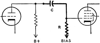
Fig. 6 - A resistance-coupled amplifier.
Fig. 7 - Basic diode detector circuit.
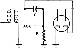
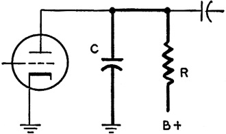
Fig. 8 - Diode circuit for agc takeoff.
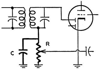
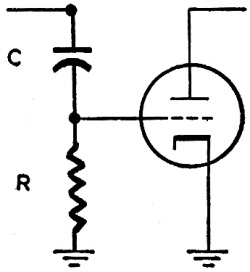
Fig. 9 - Circuit for grid-leak biasing.
Fig. 10 - A basic sawtooth generator.
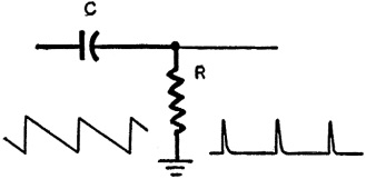
Fig. 11 - Simple differentiator network.
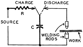
Fig. 12 - An electronic spot welder. Time constants are easy to compute. All you need do is multiply the number of microfarads capacitance by the number of megohms resistance. The product is the time constant in seconds or in fractions of a second. The scope traces of Figs. 3-a and 2-b are alike because the time constants are equal, both being 0.000048 second. Traces 3-b and 2-d are alike for the same reason - both time constants are 0.00048 second. Short time constants mean quicker charge and discharge, long ones mean slower charge and discharge rates. Here is something rather strange - applied voltage has no effect on a time constant. If we double the applied voltage used for Fig. 4-a, the charge and discharge become as 4-b. Naturally, the charge is greater than before. But because capacitance and resistance have not changed, the time for reaching 63.2% of full charge and for losing 63.2% of the charge does not change. If the applied voltage is reduced to half that used for Fig. 4-a, we have the charge and discharge of Fig. 4-c. Although full charge is now relatively small, the time for reaching 63.2% of full charge is the same as before be-cause capacitance and resistance are the same as before. Frequency has no effect on the time constant of any given capacitance and resistance. However, any change of either time constant or frequency with respect to the other may have great effect on circuit performance. Frequency effects are illustrated in Fig. 5. In 5-a the frequency of the applied voltage is such that there is practically full charge and full discharge within about half the time period of each value of applied voltage. The capacitor remains charged or discharged during the remainder of each period. If the frequency is lowered, we have the condition of 5-b. Portions of the trace showing the beginnings of charge and discharge have not changed in form but the capacitor remains charged or discharged for longer times during the longer periods of applied voltage. If the frequency is raised, as in 5-c, the periods of applied voltage are shortened. The beginnings of charge and discharge have not changed because capacitance and resistance have not been changed. But periods of maximum and zero applied voltage are so short that there is not time for full charge before discharge begins nor for complete discharge before the next charge begins. Selecting a time constant Effects of time constants on circuit performance and some of the requirements to be satisfied in selecting time constants can be illustrated by a few examples. Consider first how stage gain is affected by the time constant of capacitor C and resistor R in the resistance coupling of Fig. 6. Although there is amplification in the tube, there is loss of attenuation in the coupling and stage gain depends on both factors. Since the right-hand tube has fixed bias, grid resistor R probably must not exceed 100,000 ohms or 0.1 megohm. Were we to use 0.01-μf capacitance at C the resulting time constant would be 0.001 second. With this combination of capacitance the coupling loss would be about 5.5 db (nearly 50%) at 100 cycles. With 0.05 μf, for a longer time constant, the loss at 100 cycles becomes less than 1 db, or only about 10%. What about low-frequency cutoff, usually defined as the frequency at which gain drops to 0.707 of maximum? The cutoff frequency may be found from dividing 0.16 by the time constant. Dividing 0.16 by .001 (our time constant) shows that cutoff occurs at 160 cycles. For any lower cutoff frequency we would need a longer time constant, which might be provided by a larger capacitance at C. The time constant affects phase shift, especially at low frequencies. With 0.01- μf capacitance and 0.1-megohm resistance, for a time constant of 0.001 second in Fig. 6, the shift for signals at 100 cycles will be about 680°. Shift is lessened by a longer time constant. Changing to 0.05-μf capacitance for a time constant of 0.005 second would make the shift less than 180 at 100 cycles. In the resistance coupling we have had to juggle capacitances to change the time constant because resistance is fixed by the manner in which the tube is biased. Were we to use cathode bias the resistance at R might be as great as 0.5 megohm. With five times the original resistance we could obtain the same time constants with only one-fifth as much capacitance as previously mentioned. In the diode detector circuit of Fig. 7 the time constant is determined by capacitor C and load resistor R which here is a 500,000-ohm (0.5-megohm) volume control pot. If signal modulation as great as 80% is to be detected without distortion, the time constant should be no longer than found from dividing 0.2 by the highest audio frequency. Otherwise, the capacitor cannot discharge fast enough to follow the modulation. If we assume 5,000 cycles as maximum audio frequency and divide 0.2 by 5,000, we find that 0.00004 μf or 40 μμf is the maximum capacitance. Usually the shunt capacitance is made somewhat greater to increase detection efficiency, but there will be some distortion on strong modulation at high audio frequencies. In the agc setup of Fig. 8 the time constant must be long with respect to the time period of one cycle at the intermediate frequency, to maintain control voltage close to the amplitude of incoming signals. But capacitance C should be small to prevent taking too much signal energy from the if amplifier. To obtain a long time constant with small capacitance we need a large resistance at R. For grid-leak biasing in Fig. 9 the time constant must be considerably longer than the period of one cycle at the lowest signal frequency. Furthermore, capacitance should be so large and its reactance so small at this signal frequency that excessive attenuation is avoided. Then the time constant must be based on signal frequency and large capacitance, using resistance to suit. For the sawtooth sweep oscillator of Fig. 10 the time constant must be such that charging does not extend too far onto the bend of the curve. That is, we want a sawtooth waveform somewhat as in Fig. 5-c, not a flat top as in 5-b. In the differentiating filter of Fig. 11 we need a short time constant. The capacitor must charge very quickly and discharge just as fast. Then, even though an applied voltage such as a sawtooth drops rather slowly, there will be only brief rises and falls or only pips of filtered voltage. For electronic spot welding, an industrial application, each weld requires momentary current of several amperes, but we use a source furnishing only milliamperes. The long-time-constant circuit of Fig. 12 does it. A small current from the source, flowing for the entire period between welds, builds up a large charge in a big capacitance. Then all the stored electricity is discharged almost instantly to make a weld.
Posted October 11, 2022 |
|