"L" Networks for Reactive Loads
|
|
"L" networks are probably the most common types of impedance matching networks not just for antennas, but for an relatively narrowband load. Determining the required values for the network is relatively simple using well-established equations. Knowing how to use a Smith Chart makes the job even easier. This article from a 1966 edition of QST magazine presents the equation approach. If you have access to the May 2013 edition of QST, there is a complimentary article on L networks that uses the free Smith Chart cross-platform Java software called SimSmith. If you want to do a little complex number math, try the 1966 approach. L Networks for Reactive Loads
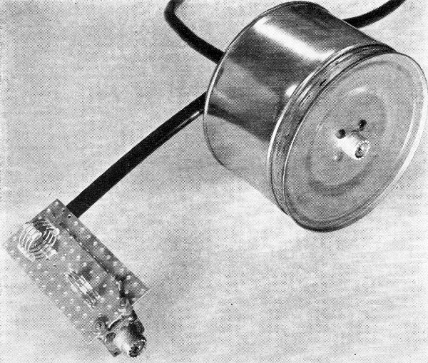
Two L networks designed by the author. To the right, the 3950-kc. network sketched in Fig. 4 is shown enclosed in a coffee can. The 14-Mc. network to the left was photographed before mounting in a similar shielding enclosure.
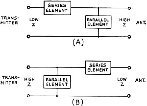
Fig. 1 - L-network configurations, (A) for stepping up the input impedance, (B) for stepping the input impedance down. Calculation for Matching Antenna System to Transmitter The usual L-network formulas for transforming an antenna-system impedance to a value appropriate for the transmitter assume that the antenna impedance is a pure resistance. The author observes that this condition seldom occurs in practice, and proceeds to discuss the more prevalent case of a complex antenna load. An article by W8CGD in an earlier issue of QST1 describes an inexpensive device for measuring antenna or other complex impedances, with ample accuracy for most purposes. I have made use of it in designing L networks to transform odd antenna impedances to the 50-ohm resistive load my transmitter prefers. The Handbook formulas for the design of L networks are limited to cases of transforming pure resistances. Unfortunately, a feed-point impedance which contains no reactive component is about as rare as a dodo. Accordingly, I derived formulas for transforming any load impedance to a pure resistance of any desired value. The L network has two possible configurations. When the resistive component of the load is greater than the desired generator resistance (RO>RI), the parallel element will be on the load side, as shown in Fig. 1A. Conversely, when the resistive component of the load is less than desired generator resistance (RO<RI), the parallel element will be on the generator side, as shown at B. In the case of a load resistance equal to the desired generator resistance it is not necessary to use the formulas, since it is apparent that compensation will be required for the reactive component only and this may be obtained by a single series clement having the same numerical value of reactance as that contained in the load, but of the opposite sign. For example, if we wish to present a 50-ohm resistive load to the transmitter, and the antenna impedance measures 50 - j30 (capacitive), we would place an inductor of reactance +j30 in series with the antenna. The transmitter will now see 50 - j30 + j30, or simply 50 ohms, resistive. The formulas for the two networks of Fig. 1 are different, so we will look at them one at a time, and work out an example for each. In all of these formulas, the subscript I refers to the input resistance of the network, O to the output impedance of the network, and S and P to the series and parallel network reactances, respectively. Hence, if we are trying to match a transmitter to an antenna, RI represents the desired resistive load we wish to present to the transmitter, and RO + jXO represents the actual antenna impedance which we have measured. Two L networks designed by the author. To the right, the 3950-kc. network sketched in Fig. 4 is shown enclosed in a coffee can. The 14-Mc. network to the left was photographed before mounting in a similar shielding enclosure.
Fig. 1 - L-network configurations, (A) for stepping up the input impedance, (B) for stepping the input impedance down.
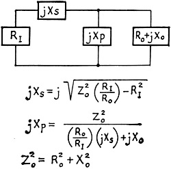
Fig. 2 - Formulas and configuration for the case where the resistive component of the load impedance is smaller than the desired load for the transmitter.
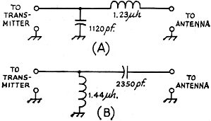
Fig. 3 - Inductive and capacitive elements in an L network may be transposed with suitable changes in values, as discussed in the text. Values shown here are for the author's case of transforming a measured 17 - j6.5 antenna load at 3950 kc. to 50 ohms resistive for the transmitter.
Fig. 4 - Sketch showing the construction of the network of Fig.3A.
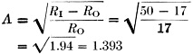
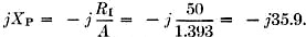
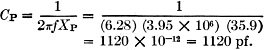
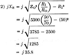
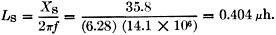
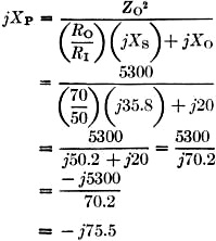
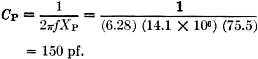
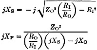
Fig. 5 - Configuration and formulas for an L network for the case where the resistive component of the load impedance is larger than the desired load for the transmitter. The Step-Down L Network We will start with the case where the resistive part of our load (RO) is less than the desired input resistance (RI). See Fig. 2 for the network sketch and formulas. The factor A has been introduced to simplify the arithmetic. My transmitter, which is designed to operate into a 50-ohm resistive load, would not tune up to the antenna on 3950 kc. Measurement on the antenna using W8CGD's device showed the reason: a measured impedance of 17 - j6.5. Here is how we proceed to design the required L network: RI = 50 ohms RO = 17 ohms jXO = -j6.5 ohms 1) 2) jXS = - jXO + jROA = j6.5 + j(17)(1.393) = j30.2 3) The plus sign tells us that the required reactance is inductive. The inductance required to yield a reactance of 30.2 ohms at 3950 kc. is then: 4) 5) The minus sign tells us that this reactance is capacitive. The capacitance required to provide a reactance of 35.9 ohms at 3950 kc. is: The circuit is then as shown in Fig. 3A. Now, on to the junk box. It produced a 1000-and a 200-pf. mica capacitor, and a piece of 5/8-inch 16-pitch coil stock. The Handbook graph says 10 1/2 turns of this will come pretty close to 1.23 µh., and the capacitance is pretty close to what we need. Adding one coffee can, coax and connectors, and a couple of hours in the cellar, produced the object shown in the sketch of Fig. 4 and the photo. With this network patched into the antenna lead, the previously-reluctant transmitter now loads without difficulty from 3900 to 4000 kc, Before leaving this topic, it should be mentioned that there is also another pair of reactance values which would do the same job if the inductive and capacitive elements are transposed. The values required may be computed in the same manner as given in the example, but using these formulas: jXS = - -jXO - jROA jXP = - -jRI/A where A has the same meaning indicated earlier. Using the data of the foregoing example, these formulas yield results as follows: jXS = - j17.2 CS = 2350 pf. jXP = j35.9 LP = 1.44 µh. The circuit is as shown in Fig. 3B. A network using these values would have performed equally well, but the required components are larger, and the internal d.c. ground on the coax center conductor found in most transmitters would be blocked from the antenna by the series capacitor. It may be worthwhile to figure the values both ways, and choose the arrangement you like best. The Step-Up L Network The other network configuration (Fig. 1A) must be used when the resistive part of our load (RO) is greater than the desired input resistance (RI). See Fig. 5 for the network sketch and formulas. None of my antenna measurements produced values of RO greater than the desired RI, so I have invented some values, for the purpose of an example, as follows: RI = 50 ohms RO = 70 ohms jXO = +j20 ohms ƒ = 14.1 megacycles 1) ZO2 = RO2 + XO2 = (70)2 + (20)2 = 4900 + 400 = 5300 2) 3) 4) (It will be noticed that j was shifted from the denominator to the numerator with a change of sign. This is accomplished by multiplying both numerator and denominator by - j.) 5) As in our previous case, there is another pair of values which will also do the same job, obtainable by the following formulas: Again using our same data, these formulas yield results as follows: jXS = - j35.8 jXP = j176 CS = 317 pf. LP = 1.99 µh. A network using these values would do the same impedance-matching job as the preceding one. As a concluding comment applicable to both network configurations, I would point out that in some cases both the series and parallel elements will be of the same kind (L or C), so if you come out with this result it doesn't necessarily signal an error in arithmetic. The photograph shows the coffee-can job described earlier, together with a prototype 20-meter job which, not being canned, is more photogenic. It has since been canned to reduce undesired local radiation. This one, you will notice, required two inductors. The companion set of formulas yielded an LC combination, but Miniductor is a lot easier to trim to size than a molded mica brick. These networks have been wholly successful in enabling me to feed my NCX-5 transceiver into a trap dipole, with plenty of room to spare on the transmitter adjustment, where previously it had been impossible to achieve the manufacturer's recommended conditions of loading. I should like to acknowledge the many helpful suggestions of Doyle Strandlund, W8CGD, during the preparation of this article. Now with a few hours of effort, you can really transform the needles, noodles, and wet string to 50 + j0. Who will be the first to build an d. noodle drier? 1 Strandlund, "Amateur Measurement, of R + jX," QST, June, 1965.
Posted February 25, 2022 |
|