Why Using Spectral Domain Simulation is Vitally Important When Designing Complex RF, Microwave, and Wireless Systems (by Ed TRoy)

Note: Ed Troy, owner of Aerospace Consulting, LLC, was kind enough to offer a few of his articles for posting on RF Cafe. With more than 30 years in the electronics communications design field, Ed has a lot of valuable knowledge to impart to us mortals ;-) This third paper demonstrates why using a highly capable software simulator for system design work is essential because of its ability to predict and facilitate mitigation of system-generated problems prior to building and testing the prototype. Case in point are spurious spectral components generated by the local oscillator and SSB to PM conversion created in a frequency doubler circuit. Stay tuned for other articles…

Why Using Spectral Domain Simulation is Vitally Important When Designing Complex RF, Microwave, and Wireless Systems

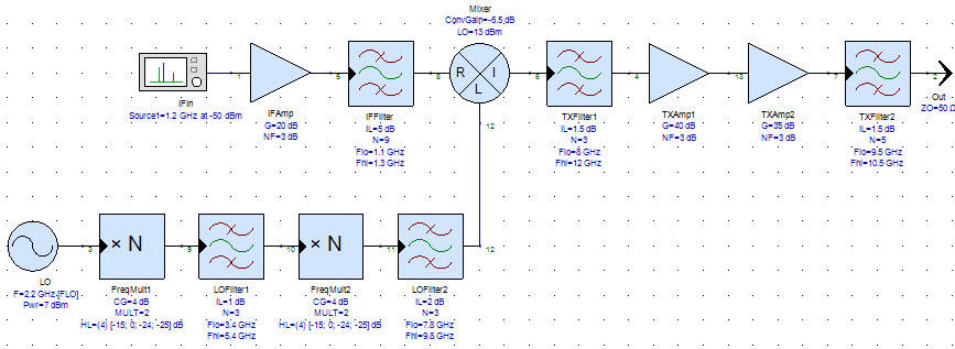
Figure 1 - Poorly designed upconverter.

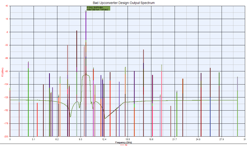
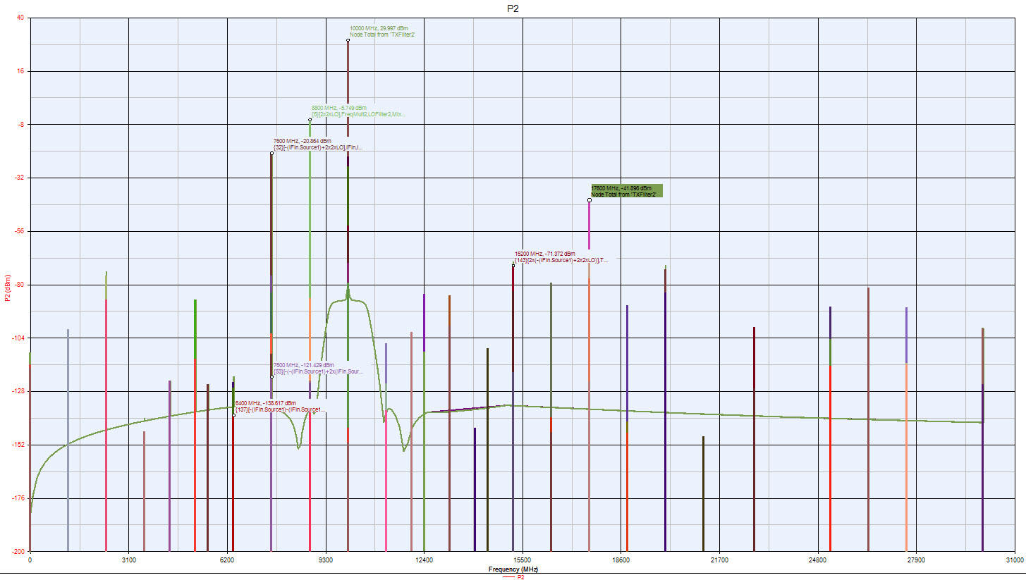
Figure 2 - Upconverter performance at output using system in Figure 1.

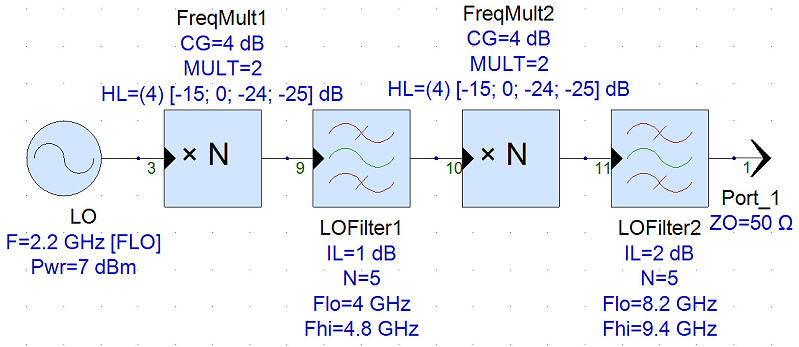
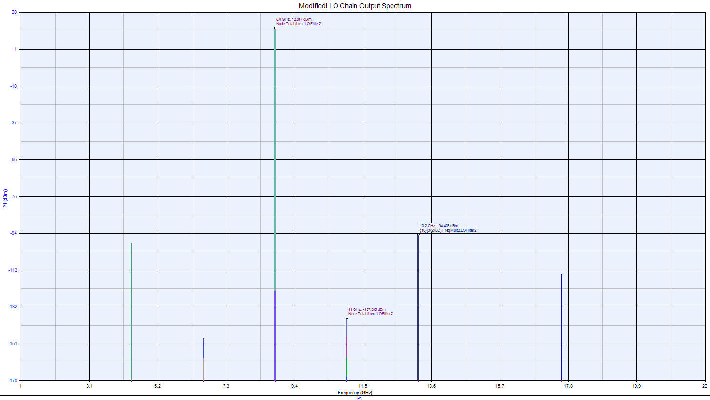
Figure 3 - Original LO Chain.

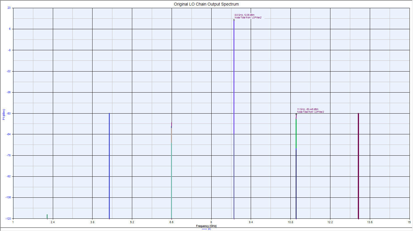
Figure 4 - Original LO chain spectrum.

Figure 5 - LO spectrum with better filtering.

Figure 6 - Spectrum of modified LO circuit shown in figure 5.

Figure 7 - Upconverter with modified LO chain.

Figure 8 - Upconverter output spectrum with modified LO chain.

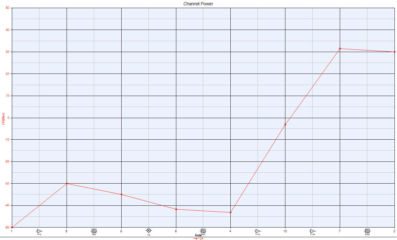
Figure 9 - Channel power level diagram for upconverter.

Figure 10 - Upconverter block diagram with modified LO and narrow TXFilter1.

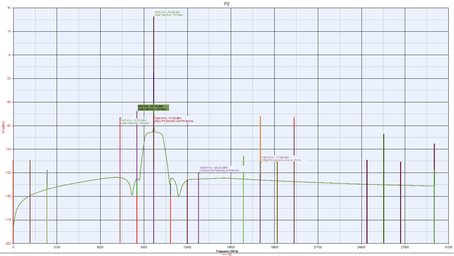
Figure 11 - Response of modified upconverter as shown in figure 10.

Figure 12 - Final system spectrum.

This paper was adapted from an example circuit provided in Keysight (formerly Agilent) Genesys Spectrasys. Spectrasys is a spectral domain block diagram simulator that allows the user to construct a system model and quickly determine the system performance. Whether you are involved in RF design, microwave design, or analog circuit and system design, Spectrasys is an essential design tool if the goal is rapid time to market and cost effective design. It is similar, in many ways, to Matlab Simulink, but Spectrasys is tailored to RF and microwave circuits and systems, rather than general systems, as is the case with Simulink. (Although Mathworks does sell modules for Simulink that are tailored to RF and microwave circuit and system design and simulation). Unlike most simulators that engineers are used to using, Spectrasys works in the frequency domain and outputs frequency spectrum components, rather than simple waveforms. This makes it ideally suited to predicting the performance of systems that combine various signals, mixers, filters, noise sources, synthesizers, and actual channel propagation models. It also has the flexibility to use generic blocks for things like filters, mixers, amplifiers, frequency sources and most other common blocks involved in RF and microwave circuit and system design, but it also allows the user to insert models consisting of actual measured (or simulated) circuit performance. For example, if you have designed an LC filter for your application, you can load the measured or simulated s-parameters of that filter into your Spectrasys model, rather than simply putting in a filter block diagram that roughly approximates your filter. This feature is extremely useful since real filters, amplifiers, mixers, and other components don't work as a simple model would imply. Using measured or simulated blocks, rather than generic blocks, allows your simulation to take into account such things as the frequency response of a real amplifier, or the varying input and output return loss. Additionally, SAW filters, while having very nice characteristics over a relatively narrow band, are often not well behaved over wider frequency ranges. With Spectrasys, you can enter a generic, sharp filter to represent a SAW filter, but you can also actually measure the filter, over many GHz if you want, and enter those measurements into the system simulation to get a much more accurate simulation. This much more accurate simulation may tell you that you need to add additional filtering, which may be as simple as an additional low pass filter, but that information could save you an entire design iteration! After all, if you don't properly account for the performance of a given component, like a SAW filter, and find out that it does not have the degree of out-of-band rejection that you had assumed, you may find that you need to add additional filtering after you have built the first prototype. Ouch!

In this paper, we start with an example provided with the Genesys package which is a design for an upconverter. The upconverter takes a signal centered at 1.2 GHz and upconverts it to a frequency between 9.5 and 10.5 GHz. The exact, final frequency is determined by the LO which is nominally at 2.2 GHz. Figure 1 shows the block diagram for this system. It consists of the input signal generator at 1.2 GHz, an LO at 2.2 GHz, 2 multipliers (x2 each), a mixer, and a number of amplifiers and bandpass filters. The goal is to take the -50 dBm source signal, at 1.2 GHz and upconvert it to 10 GHz with a power level of about +30 dBm, or 1 watt.

There are a lot of problems with this design, especially given the circuits that are available, today, for performing such designs. This design is something that might have been used 25 or 30 years ago, when the available technology was much more limited. But, it is a good example for showing the power of Spectrasys. Since it is a block diagram simulator, like Keysight (formerly Agilent SystemVue), it is very easy to use and it does not take long to develop system models. In many ways, these two programs are similar to Matlab Simulink, but probably a bit easier and more intuitive to use.

Figure 2 shows the expected output from this system. The only desired signal is the signal at 10 GHz, at about +30 dBm, with the marker.

Realistically, we almost certainly do not care too much about the signals below about -80 dBm, and maybe even a little higher than that. But, there are clearly a number of signals that are very problematic.

The signal that is especially problematic is the one located at 9.8 GHz at a level of about -33 dBm. This signal is especially problematic because it is within the pass band of the TXFilters and thus cannot be filtered. Other signals that are problematic are the ones at 8.8 and 7.6 GHz. There are other signals at somewhat lower levels that may, or may not, be problems. But, where are these signals coming from? Hovering the mouse over the signal at 8.8 GHz, the software tells us that the signal is coming from LOx2x2. Thus, it is the LO signal at the input to the mixer. Hovering the mouse over the signal at 9.8 GHz tells us that this is the result of what is called SSB to pm conversion and is related to the doubler chain. However, if we had not done a Spectrasys analysis, we would probably not have found this problem until after we built and tested the prototype! After all, our LO is at 8.8 GHz, and we have bandpass filters in the multiplier chain, so there should not be a problem, right? Wrong. Even though the primary signal at the LO port is the desired 8.8 GHz signal, we do have other frequencies present. Even though they are at a level that is significantly reduced from the desired 8.8 GHz signal, they are important.

Figure 3 shows the circuit for just the LO chain, and figure 4 shows the output of this chain, which is the input to the mixer LO port in figure 1.

In figure 4, we clearly see the desired LO signal at +12 dBm. We do see other spurious signals, but they are at a level of -50 dBm. While we might think that they would not matter, because they are 62 dB below the level of the desired LO, we would be wrong. The problematic, inband spurious signal that we see at 9.8 GHz is the result of a mix between the spurious LO signal at 11 GHz and the input IF signal at 1.2 GHz. (11-1.2=9.8 GHz).

We can show that this is true by narrowing up the passband of LOFilters 1 and 2, and increasing their order from 3 to 5. Figure 5 shows the new configuration of the LO chain, and figure 6 shows the output spectrum of the new LO chain.

Clearly, this is a much cleaner spectrum. In fact, the graph had to be rescaled to even show the spurious signal at 11 GHz. Now, it is at a level of -138 dBm, or almost 150 dB below the level of the desired LO. Of

course, this is such a low level that it would not even show up on a spectrum analyzer if someone was trying to make this measurement.

We modify the LO chain shown in figure 1 and rerun the simulation. The new model is in figure 7 and the resultant simulated spectrum is in figure 8.

Clearly, we have eliminated the inband spurious signal. But, our system still has problems. We see the LO leakage at -5.7 dBm, the image at 7.6 GHz at -21 dBm, and the second harmonic of the LO at 17.6 GHz at -42 dBm. There are other spurious signals, but they are at a low enough level that they would not

be a problem in most systems, but that does depend on the system and the regulations under which the system must operate. But, the mentioned spurious signals must be lowered.

There are a number of reasons that these spurious signals could be at such a high level. One is that the TXFilters in the output path are not sufficiently narrow or sharp. Another possibility is that the amplifiers in the output path are being over-driven and thus generating spurious and harmonic signals.

The easiest way to answer these questions is to start with the amplifiers and run a power level analysis on the system to see what the input and output power is for each of the amplifiers in the output chain. This is shown in figure 9.

From this level diagram, you can see that the amplifiers are not causing any problems. This is because the 1 dB compression level of TXAmp1 is 30 dBm and the 1 dB compression level of TXAmp2 is 50 dBm, while the output power of these amplifiers is about -3.1 and +32 dBm respectively. (These levels can be determined from the Channel power graph and the specified 1 dB compression levels are defined in the system block diagram in figure 7.)

So, that leaves the TXFilters as the culprit. A quick look at the filter specifications for TXFilter1 and TXFilter2 show that the fact that TXFilter1 is so wide that it is probably the problem. It has a lower passband edge of 8 GHz, which is below the frequency of the LO, and thus will offer no attenuation of the LO. The only attenuation that is afforded by this design is what is in the LO to IF isolation. Also, this

filter is only a 3 pole filter, and so it does not afford much attenuation. The final output filter, TXFilter2 is a bit better, but they are not good enough.

So, first we will change TXFilter1 to have the same passband as TXFilter2. That schematic is shown in figure 10. The resultant spectrum is in figure 11.

This is clearly a big improvement. In fact, at this point, the only signal that is probably still problematic is the LO leakage at a level of -24 dBm. All other spurious signals are below -68 dBm. So, we need better output filtering. We will change TXFilter1 from 3 poles to 5 poles. The spectrum of that system is shown in figure 12.

Finally, we have an acceptable system. The highest spurious level is the LO leakage at about -66 dBm. Other spurious signals are at a lower level. If more attenuation of spurious signals is needed, more filtering could be applied, or a mixer with less LO to IF leakage could be used.

The important thing is that we did not have to build a system to determine that it would not work as we desired. We were able to very simply simulate the system and make quick changes to the design to determine the necessary specifications for the various components in the system. And, by performing this system simulation, we found out about a critical inband spurious signal at 9.8 GHz that no level of output filtering would reduce. And, this signal at 9.8 GHz was almost certainly not spurious signal that we would have suspected, without the simulation, because the level of the LO signal that was causing the problem was less than -50 dBm and more than 62 dB below the level of the required LO

Aerospace Consulting was started in 1982 as a part-time business. The founder, Ed Troy, had just changed jobs from working for a company that made telemetry transmitters and other military communications equipment to a company that produced electronic article surveillance equipment. While working at ICI Americas, Ed had an opportunity to do some design consulting with a company in New York that made hardware related to anti-submarine warfare. Additionally, Narco Avionics needed help in redesigning some DME hardware because the transistor used in their high power pulse transmitter was no longer available and a new amplifier had to be designed and developed. With permission from ICI America's management, Ed started consulting on a part-time basis for these companies that were clearly not competitors of ICI's EAS business. At the same time, Ed, a pilot with commercial, multi-engine, and instrument ratings, was brokering aircraft in his free time. So, given the work for 2 aerospace-related companies and the fact that he was brokering aircraft, Aerospace Consulting seemed a natural name for the company. Today, it might seem a bit of a misnomer since most of Aerospace Consulting's customers are not aerospace companies (although some are), but the name has not been changed. In the 25 years since going full-time, Aerospace Consulting has grown dramatically both in terms of capabilities as well as the types of businesses served. Aerospace Consulting also works with companies, both large and small, that have plenty of RF, microwave, and wireless facilities and employees, but they just need some extra help to get through an especially busy time.