Computing with Scattering Parameters |
|
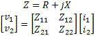
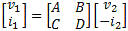
Sunshine Design Engineering Services See list of all of Joe's articles at bottom of page. Computing with Scattering Parameters By Joseph L. Cahak Copyright 2013 Sunshine Design Engineering Services Complex Numbers and Parameters A complex number is represented by two values X and Y, as in X + iY = Z. X is the real component and iY is the imaginary component with Z being the complex representation. The letter 'i' is used to designate the complex operator (√-1) by scientists and mathematicians, but in engineering the letter 'j' is most often used. This is used to represent AC or RF signals. X may be the resistance and Y the reactance in ohms of the component to an AC signal. A standard RF load for instance is represented by 50 ohms real resistance and some reactance with good loads having reactances of close to 0 ohms. X + iY can also represent a voltage and current as a function of time. Current is a function of the load and the voltage applied, so the resistances, voltages and currents are all important in describing a network for DC and AC (or RF) signals. A 2-port network can be represented by two equations with four parameters. The four parameters have different representations depending on what is known and what operations the users desire to use them for. Some network parameters (ABDC, S-, Z-, Y-, h-, etc.) are better than others depending on circuit types and the operations on them. Complex Values Complex numbers are used in a variety of ways in calculations. Typical data structures are data clusters and groups of values and the properties associated with them. Properties most often used are units of dB/linear, degrees/radians, rectilinear/polar. With this data description we know enough about the state of the complex value to operate on it for RF operations. Values in dB or dBv must first be converted to Linear and Rectilinear for most complex operations other than simple addition or subtraction. S-parameter and any other complex number must first be to converted to the proper non-decibel data format for the calculations, and then back to the final display format (dB-Polar, for instance). Z Parameters Open circuit impedance parameters are used to represent the impedances of the network. The values are complex and represent real resistance (R) and reactance (jX) of the elements of the network.
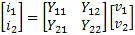
Y Parameters Short circuit parameters or admittance parameters are used to represent the inverse of impedance. The real and imaginary parts are conductance (G) and susceptance (jB). The units are mhos or Siemens.
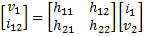
h Parameters Another model commonly used to analyze BJT (bipolar junction transistor) circuits is the h-parameter model, closely related to the hybrid-pi model and the y-parameter two-port model, but the h-parameter model uses input current and output voltage as independent variables, rather than input and output voltages. In this case it is a hybrid of an open circuit on the input and a short circuit on the output.
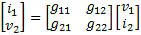
g Parameters Often this circuit is selected when a voltage amplifier is wanted at the output. The off-diagonal g-parameters are dimensionless, while diagonal members have dimensions the reciprocal of one another.
ABCD or T Parameters ABCD-parameters are known variously as chain, cascade, or transmission line parameters. This is useful for cascading 2-port network responses.
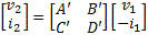
ABCD' or T' Parameters These are the inverse of the ABCD or T-parameters, respectively. They are useful for de-embedding 2-port network responses when multiplied with the ABCD matrix for the overall network.
Network Transforms
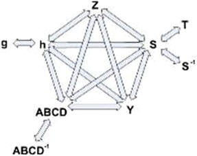
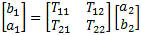
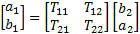
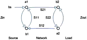
Figure 1. Network Description Transformations These are the matrix transform that are used to convert from one network description to another. Typically the –parameter, Z, Y, h and ABCD are direct conversions. The conversion to a few of the others are after the base conversion then the conversion from h to the inverse g, ABCD with the inverse ABCD-1 and S-parameter to the T (one of the two types) or the anti-S parameter (S-1) . Note that the ABCD matrix is also known as a “T” matrix; this is not to be confused with the other two descriptions of a “T” matrix connected with the S-parameters calculations and will be presented in another paper. See Figure 1 for a graphical representation of the transformations available. Transmission Lines Some of the transmission line functions and parameters are complex in value. They are excited by RF signals with most having complex modulation applied to them. Some basic measurement parameters need to be defined. A load can be represented at RF frequencies as a real resistance and an imaginary reactance driven by the charge delay or advancement as related to the driving voltage. This complex impedance is written as Z(ohms) = X + iY, with Z being complex value of the real (X) and imaginary (Y) components. Y is positive for an inductive element and negative for a capacitive element. Scattering Transfer or T-Parameters While S-parameters are useful for measurements and describing network response, it is not as useful for network embedding and de-embedding. To perform these operations another network parameter better suited: either the T-parameter or ABCD matrix. The scattering transfer parameters or T-parameters of a 2-port network are expressed by the T-parameter matrix and are closely related to the corresponding S-parameter matrix. The T-parameter matrix is related to the incident and reflected normalized waves at each of the ports as follows: b1=T11a2+T12b2 a1=T21a2+T22b2
They can be defined another way:
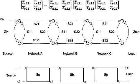
Figure 2. Cascaded Network
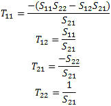
When I was researching this for the RFCalculator™ and S- parameters library, I made the discovery that there were two different definitions for these T-parameters. The RF Toolbox add-on from MATLAB and several other references use the last definition and the operations do not mix. The "From S to T" and "From T to S" in this article are both based on the first definition. Adaptation to the second definition is trivial (interchanging T11 for T22, and T12 for T21). The advantage of T-parameters compared to S-parameters is that they may be used to readily determine the effect of cascading two or more 2-port networks by simply multiplying the associated individual T-parameter matrices together. With T-Parameters, we can perform matrix multiplication for the cascading networks operations to get the total network T-Parameters and transform back to S-parameters. See Figure 2. Ttotal = TaTbTc T-Parameters are complex just like S-parameters and there are transform equations between the two parameter types and this must be performed on all elements prior to the complex matrix multiplication. Then the Ttotal must be transformed back to S-parameters for the final answer in S-parameters. Note also that matrix multiplication is not commutative; that is, AB does not equal BA. This is very important to the cascading math. S to T: To convert from S-parameters to T-parameters the following formulas apply:
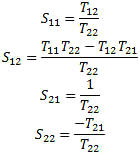
T to S: To convert from T-parameters to S-parameters the following formulas apply:
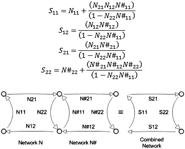
Embedding There are the formulas that can be used directly with S-parameters to embed the network response of two network components, N and N#, for the response as a singular network, S. The network embedding equation will take both network S-parameter responses and compute the S-parameters as the combined response of the two as a whole network. See Figure 3. Network Embedding Equations
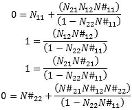
Figure 3. Embedding Cascaded Network S-Parameters S-Parameter Anti Network and De-Embedding To perform de-embedding, we must first find the inverse network or anti-network. This is done by using the embedding formula and the network to be de-embedded as one branch and the sum network to be ideal S11=S22=0 and S12=S21=1. Then, solve for the unknown sub-network to obtain the anti-network. This can then be used to embed to the network to be de-embedded to remove that network element from the total response for the sub-net response of the remaining component. See Figure 4. S11 = S22=0 and S21 = S12=1
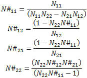
Figure 4. Anti-Network Computation Anti-Network Equation Solving for N#xx gives:
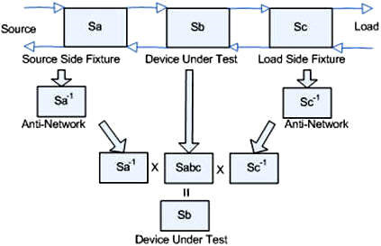
De-Embedding The process used to de-embed a sub-network from the network to get the remaining sub-network result is to calculate the anti-network of the sub-network you are removing and then cascading the result with the network to remove it from the response. Doing so produces the desired sub-network. Fixture Embedding and De-Embedding Process
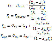
Figure 5. Fixture De-embedding Process This section describes the process of fixture embedding and de-embedding. The embedding function is included to facilitate making simulated networks to test the fixture de-embedding process. This case is an extension of the de-embedded AB network. Instead of just computing AB x A-1 = B , double up the math to compute AB and then (AB)C to get the total. The operations must be performed in the order shown in Figure 5 to be correct. 1.1.1 Gamma In and Out This value of gamma (reflection coefficient) represents the source and load impedance compared to the measurement system impedance. It gives a measure of power reflected. The gamma in and out values are both representative of the source or load looking through a network. So the gamma in is the combined response of the source and an intervening network and similarly for gamma out on the load side.
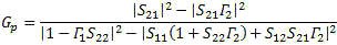
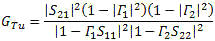
1.1.2 Gain Equations The network S-parameters can be used to calculate the scalar gain of the network. The gains are the operating power gain, transducer gain, unilateral transducer gain and the available gain. Operating Power Gain The operating power gain is the ratio of the power delivered to the load and the power input to the network.
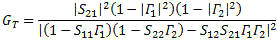
Transducer Gain Transducer gain is the ratio of the power delivered to the load to the power available from the source.
Unilateral Transducer Gain The unilateral transducer gain is the ratio of the power delivered to the load to the power available from the source for a device with little to no S12 reverse transmission (high isolation).
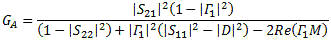
Available Gain Available gain is the ratio of the power available from the 2-port network to the power available from the source. This gain is useful to calculate the network gain (or loss) of an input network to a device being tested for noise figure. This loss is the noise figure in dBF of the input network for the cascaded gain equation when making a device noise figure measurement.
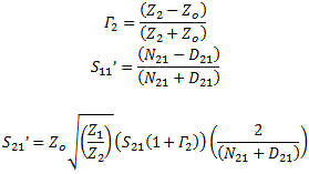
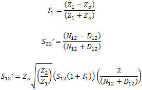
with D = S11S22 - S21S12 M = S11 - DS'22 N = S22 - DS'11 S-Parameter Re-Normalization When using a vector network analyzer (VNA), a spectrum analyzer (SA), or vector signal analyzer (VSA), the measurement impedance is defined by the system hardware which is designed to a specified system impedance. When a component must be designed and measured with an impedance not at the typical 50 ohm measurement system impedance, special accommodations must be made. In a scalar measurement system, this can be accommodated with a simple voltage impedance conversion and gain adjustment. In a complex signal environment this has to be done through the use of complex mathematical operations to account for all the complex impedances, matches and gains. I found the following formulas (see references) for the conversion of 50 ohm or any other impedance measurements to any device impedance like 75 ohms commonly found in commercial broadcast equipment or the less common video 90 ohms. The newer model VNAs have these capabilities built in. In those cases where you do not have the feature built in, these normalization formulas let you use a 50 ohm VNA to make measure an arbitrary impedance a 75 ohm amplifier measurement, for instance. See Figure 6.
Figure 6. S-Parameter Re-Normalization to Arbitrary Impedances Forward Parameters N21 = Zo[(1+S11)(1-S22Γ2)+S12S21Γ2] D21 = Z1[(1-S11)(1-S22Γ2)-S12S21Γ2]
Reverse Parameters N12 = Zo[(1+S22)(1-S11Γ1)+S12S21Γ1] D12 = Z2[(1-S22)(1-S11Γ1)-S12S21Γ1] Conclusion Shown was that S-parameters can be used for a variety of network computations and can add value to measurements where the equipment is limited in features. The reader can find these equations and more in my S-Parameter Library (DLL & LLB) and my RF Calculator products. Sunshine Design Engineering Services is located in the sunny San Vicente Valley near San Diego, CA, gateway to the mountains and skies. Are you looking for new things to design, program or create and need assistance? I offer design services with specialties in electronic hardware, CAD and software engineering, and 25 years of experience with Test Engineering services in RF/microwave, transceiver and semiconductor parametric test, test application program development, automation programs, database programming, graphics and analysis, and mathematical algorithms. See also: - Noise and Noise Measurements - Measuring Semiconductor Device Input Parameters with Vector Analysis - Computing with Scattering Parameters - Measurements with Scattering Parameters - Ponderings on Power Measurements - Scattered Thoughts on Scattering Parameters Sunshine Design Engineering Services 23517 Carmena Rd Ramona, CA 92065 760-685-1126 Featuring: Test Automation Services, RF Calculator and S-Parameter Library (DLL & LLB)
Posted August 11, 2013 |