Efficiency Measurements of Portable-Handset Antennas

Using the Wheeler Cap

Related Pages on RF Cafe

- Antenna Patterns

- Antennas - Hardware & Controls

- Antennas - Manufacturers & Services

- Test Equipment & Calibration - Antenna Measurement

- Antenna Introduction / Basics

- Antenna Radiation Patterns

- Antenna Near Field

- Near-Field / Far-Field Transition Distance

- Intro to Wave Propagation, Transmission Lines, Antennas

- Antenna, Electromagnetics & X-mission Line Simulators

- Satellite Communications - Antennas

- Short Wire Antennas

Authors:  Darioush Agahi, William Domino

 Conexant Systems Inc.

Newport Beach, CA

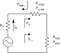
         Both authors now work for Skyworks Solutions Inc.

In the design of wireless portable devices, antenna efficiency is a variable that can have a great effect on overall system performance, and yet may not always receive the attention it deserves. As an example, RF engineers must frequently make critical tradeoffs in receiver design in order to improve sensitivity by mere fractions of a dB, but a poor antenna efficiency can easily cause a degradation of several dB. This pitfall can occur in systems such as GSM, where many tests are performed using a cable connection to the antenna port; a handset may easily pass such tests, only to be later hampered by its antenna in the field. This paper is targeted at the very important parameter of antenna efficiency, and a measurement technique that can be used to quantify it.

Antenna “efficiency” must be distinguished from antenna “gain”. Antenna gain is a directional quantity that refers to the signal strength that can be derived from an antenna relative to a reference dipole. Efficiency, on the other hand, quantifies the resistive loss of the antenna, in terms of the proportion of power that is actually radiated versus the power that is first delivered to it. It is not a directional quantity.

We model the antenna's loss as a resistor placed in series with the radiation resistance, as shown in Figure 1. Since the model includes no reactances, there is an implicit assumption that the measurements must be taken at resonance. The equations to be derived later require this assumption.

Figure1  Model of Antenna Loss

The antenna efficiency (see appendix) is 

h =                             (1)

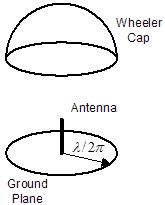
Note that it is immaterial whether the antenna is matched to the source resistance R_S. While it is certainly desirable and necessary to match the antenna in actual use, the match is not part of the problem of finding the above resistance ratio. Therefore we need only relate the radiated power to that which is transferred forward at the point shown in Figure 1. What is needed, then, is a way to effectively separate the resistances R_LOSS and R_RAD by way of measurement, so that the efficiency can be calculated.

Wheeler [1] sets forth just such a method, where a hollow conductive sphere is placed over the antenna at the radius of transition between the antenna's energy-storing near-field and its radiating far-field. This transition radius occurs at a distance of l/2p, and thus the sphere is referred to as the “radiansphere”. The role of the conductive sphere is to reflect all of the antenna's radiation while causing minimal disturbance to the near-field. In theory, a complete sphere is appropriate for reflecting the radiation of a small dipole, which is an approximation of an isotropic antenna, while in practice a monopole with a ground plane can be capped with a half-sphere. The half-spherical “Wheeler cap” is shown in Figure 2. For 900MHz, the cap's radius is 5.3cm.

Figure 2  Half-Spherical Wheeler Cap

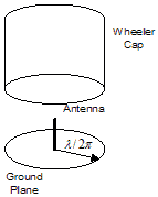
If all of the power radiated by the antenna is reflected back by the cap and not allowed to escape, then in our model this is the equivalent of setting R_RAD to zero. By making separate S₁₁ measurements with the cap in place and with the cap removed, we gather enough information to find the resistances and the antenna's efficiency.

The spherical or half-spherical cap is intended for physically small antennas; simple dipole or monopole antennas must therefore also be electrically short. Given the cap's radius, it is not possible to fit a monopole of length l/4 under it. To test such an antenna we replace the half-spherical cap with a cylindrical cap, keeping the radius at l/2p. Such a cylindrical cap is shown in Figure 3.

Figure 3  Cylindrical Wheeler Cap

For an electrically short antenna (< l/10), the radiation resistance is typically small in comparison to the 50W source resistance of the measuring system. The radiation resistance of an ideal short monopole [2] is

R_{RAD MONO} =                                (2)

So, for example, a 1/20-wavelength monopole, which fits comfortably under the half-spherical cap, exhibits about a 4W radiation resistance. With such a small value of R_RAD, the power lost in the resistance R_LOSS is about the same whether the cap is in place or removed, that is, with zero or finite R_RAD. With the assumption of constant power loss, we can make use of S₁₁ magnitude measurements with the cap on and off as follows:

Cap on. The radiation resistance is zero, and the antenna reflection coefficient is measured and referred to as S_11WC.  Then

                         (3)

Cap off. The radiation resistance is that of the antenna radiating into free space, and the antenna reflection coefficient is measured and referred to as S_11FS. Then

                            (4)

We need only measure the magnitudes (and not the signs) of S_11WC and S_11FS.  The antenna efficiency becomes

h =                              (5)

h =                                (6)

The efficiency can therefore be found directly from the reflection coefficient magnitude measurements, without any need to actually determine R_RAD and R_LOSS. It should still be noted that the measurements must be made at resonance, because the loss model is based on vector S₁₁ values that are all-real, even though only their magnitudes are needed in the above equations.

Eq. (6) appears in [3] in a survey of previous techniques. This method was likely developed to make it possible to obtain an antenna efficiency measurement using only reflectometer-type reflection-coefficient measurements, where only the magnitude of S₁₁ is measured. In this case the method further depends on the close proximity of the minimum of |S₁₁| to its all-real point.

For our example of a 1/20-wavelength monopole, suppose the measurements are

S_11WC = -0.966                      S_11FS = -0.823

Then the efficiency calculated from eq. (6) is

h = 79.3%

This antenna causes a performance penalty to the radio of

10log(79.3%)  = -1.0 dB

Such an efficiency is not atypical, and some antennas have been measured to be even less than 50% efficient, which corresponds to a power loss of more than 3dB. This power loss is a direct degradation of the receiver sensitivity and the transmitter output power, relative to a cable-connection test. Such a transmitter power loss would greatly degrade the handset's battery life, and, in cellular systems that tend to be uplink-limited, it would affect the ability of the handset to obtain service in marginal areas. In a 1/8-duty-cycle GSM system operating at full transmit power of 2W with a 50% efficient antenna, the resistive heating of the antenna would amount to 1/8W!

As the antenna becomes longer, its radiation resistance increases, and the assumption of constant power loss with and without the cap breaks down. In this case a method of efficiency measurement that directly makes use of the quantities R_RAD and R_LOSS is preferred. Fortunately, modern vector network analyzers can provide a direct display of the impedance of a measured device when performing a reflection coefficient measurement. So we make use of the resistance ratio in (1) rather than the power ratio:

h =                            (7)

Here the key assumption is that R_LOSS itself, rather than the power lost in it, remains constant with the cap in place or removed. If desired, we can still express the efficiency in terms of the reflection coefficients:

Cap on. The radiation resistance is zero, and the antenna reflection coefficient is S_11WC.  Then

                       (8)

Cap off. The radiation resistance is that of the antenna radiating into free space, and the antenna reflection coefficient is S_11FS. Then

                    (9)

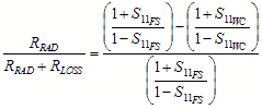
 (7) and (8) are transposed to become

                          (10)

                        (11)

And the efficiency is

h =                   (12)

h =                      (13)

Eq. (13) is actually more accurate then eq. (6) regardless of the absolute value of R_RAD (and thereby of the antenna length). Its one disadvantage lies in the fact that the signs of the (all-real) S₁₁ measurements must be retained and accounted for in the calculation, making for somewhat less convenience. But it exactly reproduces the resistance ratio at any level of antenna efficiency, as opposed to eq. (6) which becomes less accurate at lower efficiencies.

As an example, consider a low-efficiency monopole, where the S₁₁ measurements are:

S_11WC = -0.626                      S_11FS = -0.325

Then the efficiency calculated from eq. (13) is

h = 54.9% = -2.6dB

while that calculated from eq. (6) is

h = 32.0% = -4.9dB

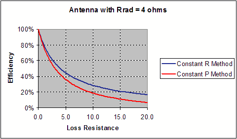
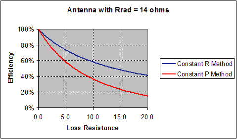
The value of efficiency calculated by the constant-power-loss method is unnecessarily pessimistic. This discrepancy between the methods occurs with longer antennas that inherently exhibit a large R_RAD.

Next we plot the calculated efficiency vs. a swept value of R_LOSS, in order to further compare the two methods of calculation. Figure 4 is plotted for an R_RAD of 4W (our short-antenna case) while Figure 5 is for an R_RAD of 14W (a longer antenna). In the 4W case the curves agree down to about 75%, while in the 14W case they quickly diverge. In either case the constant-loss-resistor method is more accurate, as it agrees with the resistance ratio. This illustrates that the constant-power-loss method is accurate only for small radiation resistances and high efficiency.

Figure 4  Efficiency vs. R_LOSS for Antenna with 4W Radiation Resistance

Figure 5  Efficiency vs. R_LOSS for Antenna with 14W Radiation Resistance

Making the Measurements: Practical Considerations

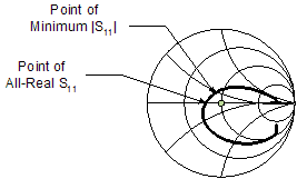
In the above derivations it was assumed that the radiation and loss resistances are not accompanied by any reactive impedances; therefore the S₁₁ measurements need to be made at  the antenna's actual resonance, as defined by the point where S₁₁ is all-real. For an ideal lossless antenna and perfectly-reflecting Wheeler cap, the S₁₁ measurements would be -1 with the cap on and zero with the cap off, and we need to find the points of all-real impedance that most closely approach these. They may or may not be precisely the

same as where the magnitude |S₁₁| is minimized, as illustrated in Figure 6, and so it is advisable to view the measurements on a Smith chart display rather than a log-magnitude grid. These points should not be too far apart.

Figure 6  Smith Chart Display of Free-Space S₁₁

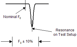
It is especially true that the free space measurement should be done at the actual resonance instead of the antenna's nominal operating frequency F₀. This is because the antenna is normally loaded down when installed on the handset, and it is expected that there should be a small shift when it is removed and placed on a different ground plane. A rule of thumb that is normally used for the maximum limit of this shift is ± 10% of F₀. De-tuning beyond this could impact the accuracy of the measurement, as it means the actual-usage environment differs too much from the measuring setup.

Figure 7  Allowable De-tuning for Measurement

Conclusion

The Wheeler cap provides a convenient and reasonably accurate method of determining antenna efficiency. For practical use it consists of a cap over a ground plane, usually of a simpler shape than the ideal half-sphere, such as a cylinder, keeping the l/2p radius. The efficiency is best determined by measurement of the antenna resistance with the cap in place and removed, each taken at the resonance defined as the all-real impedance point.

Appendix

The derivation of equation (1), which also appears in ref. [2] page 48, is duplicated here. In the ideal case, where there are no disturbances to the antenna, and a perfect match, the input resistance represents the dissipation loss of the antenna. This resistance represents the sum of radiation resistance and ohmic resistance.

R_in  =  R _RAD  +   R_LOSS                                        (a1)

Given that the peak current flowing in to the antenna is I_in then the average power dissipated in an antenna is

Pin  =   ½ R_in | I_in |²                                                   (a2)

Inserting (a1) into (a2) yields,

Pin =  ½ ( R _RAD  +    R_LOSS) | I_in |²  =  ½ R _RAD | I_in |²  +   ½ R_LOSS | I_in |²

Or equivalently,

P_RAD  =   ½ R _RAD | I_in |²                          (a3)

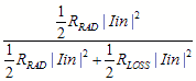
P_LOSS  =  ½ R_LOSS | I_in |²                          (a4)

Using the efficiency equation and inserting (a3) and (a4) yields,

h        =  =  =

After canceling similar terms, it yields,

h        =

References:

1) H. A. Wheeler, “The radiansphere around a small antenna,” Proc. Of the IRE, vol.47, pp.1325-1331, Aug. 1959.

2) W. L. Stutzman and G. A. Thiele, Antenna Theory and Design, Wiley, New York, 1981.

3) R. H. Johnston, L. P. Ager, and J. G. McRory, “A new small antenna efficiency measurement method,”

IEEE 1996 Antennas and Propagation Society International Symposium, vol.1, pp. 176-179

Authors:

Darioush Agahi, P.E.  is director of GSM RF systems engineering at Conexant Systems Inc. in Newport Beach CA. He has 17 years of industry experience of which the last 4 years he has been with Conexant and 9 years with Motorola's (GSM) cellular subscriber division. Darioush received his BS in electronics (1981) and MS in Medical Engineering from the George Washington University in Washington DC (1983). Also he received an MSEE from Illinois Institute of Technology in Chicago Illinois (1993) and an MBA from National University in 1997. Darioush holds ten US patents and several more pending, he is a Professional Engineer (P.E.) registered in the state of Wisconsin.

William Domino is Principal Engineer, GSM RF Systems, at Conexant Systems Inc. in Newport Beach, CA, where he has been employed since 1992 in the area of digital-radio system architecture development. He received the BSEE degree from the University of Southern California in 1979 and the Master of Engineering from the California State Polytechnic University, Pomona, in 1985. His interests currently include receiver and transmitter system design for various cellular standards, as well as filter design. In these areas he has one patent issued and ten patents pending.